Download
1 / 8
80 likes | 195 Views
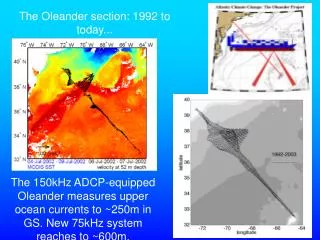
The Oleander section: 1992 to today. The 150kHz ADCP-equipped Oleander measures upper ocean currents to ~250m in GS. New 75kHz system reaches to ~600m.

E N D
The Oleander section: 1992 to today... The 150kHz ADCP-equipped Oleander measures upper ocean currents to ~250m in GS. New 75kHz system reaches to ~600m.
Example of a good weather (no bubbles) ADCP section. The data are uploaded when the vessel docks in Port Elisabeth. We are striving to serve the final product within a few days. Direct measurements of currents provide highly accurate information on currents, their structure and space-time variability. In absolute units, no assumptions about geostrophy, and/or reference velocities. cont. slope backscatter limit
The non-dimensional Ekman spiral as derived from Oleander ADCP measurements and NCEP winds and heat fluxes. The numbers indicate depth normalized by the Price-Sundermeyer Ekman scale depth. The axes are E-W and N-S velocity normalized by windstress and Ekman layer depth. Given that the actual Ekman velocities are only a few cm/s this is an impressive result! (S. Stoermer, MS-thesis, GSO/URI)
Repeat detection of an eddy Detection and quantification of coherent vortices in the SS. The main point of this figure is that repeat sampling allows for quantitative analysis of the mesoscale eddy velocity field. Distribution of core vorticity across the SS. (D. Luce, MS-thesis, GSO/URI)
Integration of velocities across the ship track gives transport in the Slope Sea, Gulf Stream and Sargasso Seas as a function of time. (Transport in 1 m thick layer at 52 m.) . The red lines highlight the GS, Slope and Sargasso Sea transports over the 11 years.
We have written that the mean path of the GS may be controlled by Slope Sea transport and thus has a thermohaline (Labrador Sea) origin, but is considered an open question. - The large variations in the Sargasso Sea very likely have a wind-driven explanation. SW NE SW
data courtesy NMFS Time-varying fluxes from the Labrador region are very likely responsible not only for path (top) but also for SSS variations. But exactly how is not clear.
At this juncture the main signal to emerge is the constancy of GS transport yet x2 variations in both the Slope and Sargasso Seas. Why is GS transport so stable but not that of surrounding waters which in part feed it? By September we will have been in operation for 15 years. This summer we plan to submit a proposal to continue for another five years. The deeper ADCP reaches well below the main pycnocline in the Slope Sea so we can measure directly upper Labrador Sea water velocities and transport. Similarly for the Gulf Stream and Sargasso Sea (600+m). This ongoing effort has been possible by the excellent cooperation of the BCL and with our NMFS colleagues across the street at home. They operate the XBT and TSG program. have been and are terrific partners.