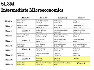
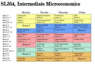
Download

1 / 24
250 likes | 474 Views
ECO 365 – Intermediate Microeconomics. Lecture Notes. Monopoly . Market environment where there is only one firm in the market Firm faces ALL of demand So monopoly profit = p(y)y – c(y) Where p(y) = inverse market demand let p(y)y = r(y) revenue function Monopolistic problem:

E N D
ECO 365 – Intermediate Microeconomics Lecture Notes
Monopoly • Market environment where there is only one firm in the market • Firm faces ALL of demand • So monopoly profit = p(y)y – c(y) • Where p(y) = inverse market demand let p(y)y = r(y) revenue function • Monopolistic problem: • Choose y to Max r(y) – c(y) • First order conditions are given by: • MR = MC
The same condition we got with perfect competition • But now MR does not equal P (i.e. firms not price takers) • Two effects of changing y (say increase y) on revenues • 1-sell more so revenue increases • 2-price decreases so revenue decreases • ∆ r (y) = p ∆y + y ∆p • ∆ r(y)/ ∆ y = MR = p + y ∆p/ ∆y or: • For price takers ∆p=0 => ∆r = p ∆y • But now P decreases as y increases so the second term matters.
Now both 1 and 2 measure Marginal Revenue (MR) • MR= ∆r/ ∆y = p + y ∆p/ ∆y • = p(1 + (y/p)(∆p/ ∆y) • = p(y) (1 + 1/ε) • Since ε = price elasticity of demand = (p/y)(∆y/∆p) • => can re-write optimal condition, MR = MC as: • p(y) (1 + 1/ ε(y)) = mc (y) • Or p(y) (1- 1/| ε(y)|) = mc (y) • Since ε < 0 • Also recall that | ε | > 0 elastic • | ε | < 1 inelastic • So that if demand elastic regions | ε | > 1 • MR > 0 but if demand inelastic MR < 0
The above implies that the Monopolist only operates in elastic portion of Demand since • MR < 0 when demand inelastic and profit max. requires MR = MC but MC < 0 is unlikely (impossible). • Now with linear demand… • P(y) = a –b y • So R (y) = ay –by2 • => MR= a – 2by • Notice 3 things: • 1. MR = D at y=0 • 2. slope of MR = 2 times the slope of demand (i.e., twice as steep). • 3. MR = 0 where | ε | = 1 (this is always true not just for linear Demand)
MC AC Pm • Look at tax example: suppose c(y) = cy • => mc = c • P(y) = a-by so MR = a -2by D MR Ym y
Now suppose a tax on the monopolist = t (quantity tax) so pc = ps + t • So mc w/ tax is c + t or c(y) = (c+ t)y • => before profit max where c = a -2by • Or y* = a-c/2b • Now MC = c + t = a – 2by = MR • So y* = (a-c-t)/2b • => Δy/ Δ t = -1/(2b) (why?) • What is the impact of the tax on price, p? • Recall slope of demand function = Δp/ Δy = -b, so • The tax is imposed => y changes by -1/(2b) then • The price changes by – b, the overall impact is both of these together, • Or – b times -1/(2b) = -1/2 • Interpretation: if t increases by $1 => price increases by $.50
But note that p may actually increase more than by the amount of tax. See book for example pt P* C + t MC = C MR D Yt y*
Now look at efficiency and compare to perfect competition • Again assume MC = C (constant returns) in the long run • Produce at (pm, ym) Pm Pc=c Deadweight loss to society MC=LRAC MR D Ym yc • But competitive firms would produce at MC = D • Or (pc, yc) which is the point that maximizes net surplus to society.
Or if upward sloping LRMC Pm Pc Deadweight loss to society MC MR D Ym yc
=> appears that monopolist is inefficient (i.e. does not max society’s net surplus) • Public policy: may be to get rid of monopolies • (1) contestable markets i.e. free entry => if profit > 0 more firms enter so profit = o even with one firm. • (2) economies of scale and scope • Consider natural monopoly (economies of scale) Pm Pt LRMC LRAC D MR Ym
Only one firm can cheaply produce given demand but • (1) if p=mc=Pso(socially optimum price) • Firms makes a loss and leaves • (2) if p=pm => deadweight loss • (3) if p=AC=pf (fair price) still a loss in profit but firm can operate • But if break up of monopoly: • Pc > Pm > Pf >Pso => competition is not more efficient due to economies of scale. • Same may to be true due to economies of scope.
Price Discrimination • 3 different types • A. Perfect price discrimination—price the monopolists sells is just equal to your willingness to pay => • With no price discrimination produce at (pm, ym) but this assumes no ability to discriminate • Now perfectly discriminate => D=MR and produce at Yc which is efficient (assuming $1 to producer is the same as $1 to consumer since CS=0) Pm Pe MC D MR Ym Ye
2nd degree Price Discrimination • Pi= f(yi) i.e. how much you pay depends on your consumption • Examples: utilities, bulk discounts for large purchases • 3rd degree price discrimination-different groups get different prices but individuals within a group get the same price • Most common type: Examples • 1. movie theatre discounts (kids v. adults) • 2. local ski discounts (locals v. non-locals) • More formally suppose 2 groups with different demand • => max P1 (Y1) Y1 + P2 (Y2) Y2 – C(Y1 + Y2) by: • MR1 – MC(Y1 + Y2) = 0 • MR2 – MC(Y1 + Y2) = 0
Combine to get MR1 = MC(Y1 + Y2) = MR2 or • P1 [1- 1/| ε1|] = MC (Y1 +Y2) = P2 [1-1/| ε 2|] • If P1 > P2 => [1-1/| ε 1|] < 1 – 1/| ε 2| or • 1/| ε 1| > 1/| ε 2| or | ε 2| > | ε 1| • i.e. for P1 > P2 demand for group 1 must be more inelastic • Graphically, assume C= MC Group 1 Group 2 P1 D1 P2 C C MR1 D2 MR2 Y2 Y1
Innovation—monopolies have more incentive to innovate (at least this is the argument) • Define innovation • Just a decrease in MC to MC2 assuming constant returns P MC1 MC2 Q
What are the incentives to innovate for monopoly? • I.e. increase profit due to innovation = shaded area. Why? P MC1 MC2 D MR Y
What are incentives to innovate for perfectly competitive industry? • None unless (1) innovative technology is secret or (2) a patent system exists • Under a patent system what is the incentive? What are increased profits to patent holder? • 1st what does patent holders MR curve look like? As long y < y* MR = C ; i.e. he’s a price taker. P MC1 C C1 MC2 D Q Y*
But if y > y* the firm becomes sole supplier • R= p(y)y so MR is downward sloping and determined by D when y > y*. • Note: as long as C > C* ; y = y* in the market. This is a small innovation. • But if C < C* so y > y* then this is a large innovation. P C C1 C* D MR Y* Y
Incentive to innovate to competitive industry • Now just look at a small innovation (i.e. y = y* before and after innovation) P C C2 D MR • Notice that the incentive to innovate for a competitive industry is greater than for a monopoly because output is larger for the competitive firm. Y
Q: What if economies of scale in innovation (i.e. small firms in competitive industry don’t have resources to innovate) • A: Firms specialize in innovating, gain patents and license to small competitive firms • Example: agriculture where innovating is done by • Universities • Seed companies • Etc.
Monopolistic Competition • Characteristics • Large numbe r of potential sellers • All small relative to market • Differentiated product • Easy entry and exit • The short-run looks like a monoply Pm MC ATC Profit MR D Ym
Profit can also be negative or zero in the short-run. If negative => firms exit if p< avc. • Long-run equilibrium is just like for competition: • If profit > 0 => entry which drives profit down. • If profit < 0 => exit which drives profit up. • Therefore, long-run equilibrium is where profit equals zero, where no exit or entry. Po Pc MC ATC Qo Qc D MR
Notice that at Equilibrium but P > MC • Resource Allocation & Efficiency • Since MSC does not equal MSB or MSB > MSC => inefficient p.c. firm would produce the efficient amount. • Might be efficient if benefit from different products > Cost of producing different products • => in long run (1) each firm is on its demand curve • (2) each firm chooses y to max profit • (3) entry forces profit = 0 • (4) P > MC => inefficient