Download
1 / 14
160 likes | 581 Views
ECO 365 – Intermediate Microeconomics. Lecture Notes. Profit Maximization . Profits ( π ) = TR – TC or π = Σ P i Y i - Σ w j X j for i = 1 to n (outputs) and j = 1 to m (inputs). Types of Firms Proprietorship – single owner Partnership – two or more owners

E N D
ECO 365 – Intermediate Microeconomics Lecture Notes
Profit Maximization • Profits (π) = TR – TC or • π = ΣPiYi - ΣwjXjfor i = 1 to n (outputs) and j = 1 to m (inputs). • Types of Firms • Proprietorship – single owner • Partnership – two or more owners • Corporation – firm is a separate legal entity • Advantages and Disadvantages • Factors of Production (Inputs) – 3 Types • Variable inputs – varies with y. • Fixed inputs – fixed even if y=0. • Quasi-fixed inputs (if y=0 then x=0 but if y>0 then x is fixed).
Short-run π maximization • Assume only 1 output Y and two inputs L & K • K is fixed => in short-run • Firm problem is to choose L to maximize: • Given that y = f(K,L) => choose L to max: • How? • MPL = w/p or p*MPL = w – what does this mean? • Graphically • Recall π = py – wL – rK, with K fixed or solve for y to get • y = π/p + wL/p + rK/p • Recall that p, w, r, and K are all fixed paramters, if we also hold π constant then we get a straight line in L, y space:
Y Slope = w/p Intercept = π /p + rK/p L
The curve in the graph above is called an iso-profit curve. Why? • Along a given iso-π then profit is fixed. • If profit ↑ (↓) then the line shifts up (down). • Thus, have a family of curves, all with same slope where profit increases as you move and decreases as you move down.
Y π↑ L L1
Y Isoprofit curve Y* L L*
Discuss the Graph above: • Maximize profit by getting on highest iso-profit curve. • Subject to constraint that must be on the production function. • => tangency between the two or • Slope of production function = slope of iso-profit or • MPL = w/p – notice that this is the same condition as we already derived for profit maximization. • What happens as P or w change? • P ↑ or ↓ => what happens to L* and Y*? • w ↑ or ↓ => what happens to L* and Y*? • Show both graphically. Hint what happens to the slope of all isoprofit lines?
The Long-Run • Maximize profit = pf(L,K) – wL – rK • Both L and K are variable and hence a more complex problem. • Recall that in the SR, profit max required MPL = w/p • In LR is this still true? • Also requires that MPK = r/p • or P*MPK = r; P*MPL = w • Both conditions must occur simultaneously • Use these conditions to derive Factor Demand curves • L* = f(p, w, r) and K* = f(p, w, r) • Substitute these into production function to get optimal output Y = f(L*, K*)
Inverse factor demand curves • w = f(L, K*, P) = P*MPL (L, K*) • r = f(L*, K, P) = P*MPK (L*, K) • or graphically – why downward sloping? w DL L
Returns to Scale • What happens to profit with constant returns to scale? • Inputs double => costs double => output doubles => profits double but => original output level was not profit max. • What happens with increasing returns to scale? • Problems • If original profit = 0 => 2*0 = 0 => original profit may have been profit max. • Eventually get decreasing returns to scale => what happens to profit? • If firm size increases (Y increases) => under what conditions will P remain constant? • Even if market competitive => if all firms increase Y => P will increase.
Revealed Profitability • What is it? • Suppose at time = t => with pt , wt, rt then the firm chooses Yt, Lt, and Kt. • At a different time = s => with ps , ws, rs then the firm chooses Ys, Ls, and Ks. • Must be true that: • (1) pt Yt - wt Lt - rt Kt ≥ pt Ys - wt Ls - rt Ks - why? • (2) ps Ys - ws Ls - rs Ks ≥ ps Yt - ws Lt - rs Kt - why? • WAPM = Weak Axiom of Profit Maximization • To be π maximization point the π from actual choices must be ≥ π from other possible choices at that time.
Implications of WAPM? • Transform equation 2 to get: • (3) -ps Yt + ws Lt + rs Kt ≥ -ps Ys + ws Ls + rs Ks • Now add equations 3 and 1 together to get: • (pt – ps)Yt – (wt – ws)Lt – (rt – rs)Kt ≥ (pt – ps)Ys - (wt – ws) Ls - (rt – rs)Ks or: • (pt – ps)(Yt – Ys )– (wt – ws)(Lt - Ls) – (rt – rs)(Kt - Ks)≥ 0 • Or (4) ΔpΔY – ΔwΔL – ΔrΔK ≥ 0 • Suppose Δw = Δr = 0 => equation 4 implies that ΔpΔY ≥ 0 => if Δp > 0 then it must also be the case that ΔY > 0. What does this mean? • Supply of the output is upward sloping
More implications of WAPM • Suppose Δp = Δw = 0 => equation 4 implies that • – ΔrΔK ≥ 0 or ΔrΔK ≤ 0 or if Δr ≥ 0 then it must be true that ΔK ≤ 0. What does this mean? • Demand for Capital is downward sloping • Do the same thing to show demand for labor is also downward sloping. • Finally, note that profit maximization implies cost minimization (producing given Y with lowest costs). Why?