Part 8 : Neural Networks

1. METU Informatics Institute Min720 Pattern Classification with Bio-Medical Applications Part 8: Neural Networks

2. 1- INTRODUCTION: BIOLOGICAL VS. ARTIFICIAL Biological Neural Networks A Neuron: • A nerve cell as a part of nervous system and the brain (Figure: http://hubpages.com/hub/Self-Affirmations)

3. Biological Neural Networks • There are 10 billion neurons in human brain. • A huge number of connections • All tasks such as thinking, reasoning, learning and recognition are performed by the information storage and transfer between neurons • Each neuron “fires” sufficient amount of electric impulse is received from other neurons. • The information is transferred through successive firings of many neurons through the network of neurons.

4. Artificial Neural Networks An artificial NN, or ANN or (a connectionist model, a neuromorphic system) is meant to be • A simple, computational model of the biological NN. • A simulation of above model in solving problems in pattern recognition, optimization etc. • A parallel architecture of simple processing elements connected densely.

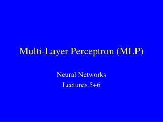
5. Y1 An Artificial Neural Net Y2 a neuron w w w w Y1, Y2 – outputs X1, X2 – inputs w – neuron weights X1 X2

6. Any application that involves • Classification • Optimization • Clustering • Scheduling • Feature Extraction may use ANN! Most of the time integrated with other methods such as • Expert systems • Markov models WHY ANN? • Easy to implement • Self learning ability • When parallel architectures are used, very fast. • Performance at least as good as other approaches, in principle they provide nonlinear discriminants, so solve any P.R. problem. • Many boards and software available

7. APPLICATION AREAS: • Character Recognition • Speech Recognition • Texture Segmentation • Biomedical Problems (Diagnosis) • Signal and Image Processing (Compression) • Business (Accounting, Marketing, Financial Analysis)

8. 1940 - McCulloch-Pitts (Earliest NN models) Background: Pioneering Work 1950 - Hebb- (Learning rule, 1949) - Rosenblatt(Perceptrons, 1958-62) 1960 -Widrow, Hoff (Adaline, 1960) 1970 1980 - Hopfield, Tamk (Hopfield Model, 1985) - RumelHart, McClelland (Backpropagation) - Kohnen (Kohonen’s nets, 1986) 1990 - Grossberg, Carpenter (ART) 90’s Higher order NN’s, time-delay NN, recurrent NN‘s, radial basis function NN -Applications in Finance, Engineering, etc. - Well-accepted method of classification and optimization. 2000’s Becoming a bit outdated.

9. ANN Models: Can be examined in 1- Single Neuron Model 2-Topology 3- Learning 1- Single Neuron Model: General Model: 1 w0 Y +1 w1 X1 +1 wN -1 -1 XN linear Step(bipolar) Sigmoid

10. - Activation function Binary threshold / Bipolar / Hardlimiter Sigmoid When d=1, Mc Culloch-Pitts Neuron: • Binary Activation • All weights of positive activations and negative activations are the same. Excitatory(E) 1 Fires only if where T=Threshold 1 1 Inhibitory(I) 1

11. Higher-Order Neurons: • The input to the threshold unit is not a linear but a multiplicative function of weights. For example, a second-order neuron has a threshold logic with with binary inputs. • More powerful than traditional model. 2. NN Topologies: • 2 basic types: • Feedforward • Recurrent – loops allowed • Both can be “single layer” or many successive layers.

12. Y=output vector T=Target output vector X=input vector A recurrent net A feed-forward net

13. 3.Learning:Means finding the weights w using the input samples so that the input-output pairs behave as desired. supervised- samples are labeled (of known category) P=(X,T) input-target output pair unsupervised- samples are not labeled. Learning in general is attained by iteratively modifying the weights. • Can be done in one step or a large no of steps. Hebb’s rule:If two interconnected neurons are both ‘on’ at the same time, the weight between them should be increased (by the product of the neuron values). • Single pass over the training data • w(new)=w(old)+xy Fixed-Increment Rule (Perceptron): • More general than Hebb’s rule – iterative • (change only if error occurs.) t – target value – assumed to be ‘1’ (if desired), ‘0’(if not desired). is the learning rate.

14. Y w X Delta Rule:Used in multilayer perceptrons. Iterative. • where t is the target value and the y is the obtained value. ( t is assumed to be continuous) • Assumes that the activation function is identity. Extended Delta Rule:Modified for a differentiable activation function.

15. PATTERN RECOGNITION USING NEURAL NETS • A neural network (connectionist system) imitate the neurons in human brain. • In human brain there are 1013 neurons. A neural net model • Each processing element either “fires” or it “does not fire” • Wi – weights between neurons and inputs to the neurons. outputs w1 w2 w3 inputs

16. 1 w0 X1 w1 Y X2 The model for each neuron: f- activation function, normally nonlinear Hard-limiter wn Xn +1 -1

17. +1 Sigmoid Sigmoid – TOPOLOGY: How neurons are connected to each other. • Once the topology is determined, then the weights are to be found, using “learning samples”. The process of finding the weights is called the learning algorithm. • Negative weights – inhibitory • Positive weights - excitatory -1

18. How can a NN be used for Pattern Classification? • Inputs are “feature vectors” • Each output represent one category. • For a given input, one of the outputs “fire” (The output that gives you the highest value). So the input sample is classified to that category. Many topologies used for P.R. • Hopfield Net • Hamming Net • Multilayer perceptron • Kohonen’s feature map • Boltzman Machines

19. y1.........................................ym MULTILAYER PERCEPTRON Single layer Linear discriminants: • Cannot solve problems with nonlinear decision boundaries x1.........................................xn x1 x2 • XOR problem • No linear solution exists

20. y1.........ym Hidden layer 2 Multilayer Perceptron Fully connected multilayer perceptron • It was shown that a MLP with 2 hidden layers can solve any decision boundaries. Hidden layer 1 x1.........................................xn

21. Learning in MLP: Found in mid 80’s. Back Propagation Learning Algorithm 1- Start with arbitrary weights 2- Present the learning samples one by one to inputs of the network. • If the network outputs are not as desired (y=1 for the corresponding output and 0 for the others) - adjust weights starting from top level by trying to reduce the differences 3- Propagate adjustments downwards until you reach the bottom layer. 4- Continue repeating 2 & 3 for all samples again & again until all samples are correctly classified.

22. Example: 1 for XOR -1 for others AND X1, X2=1 or -1 Output of neurons: 1 or -1 Output=1 for X1, X2=1,-1 or -1,1 =-1 for other combinations NOT AND -1 .7 -.4 AND GATE Fires only when X1, X2=1 OR GATE .5 -1.5 1 1 1 1 1 X1 X2

23. +1 Activation function -1 -1 .4 .7 Take –(NOT AND)

24. Expressive Power of Multilayer Networks • If we assume there are 3 layers as above, (input, output, one hidden layer). • For classification, if there are c categories, d features and m hidden nodes. Each output is our familiar discriminant function. • By allowing f to be continuous and varying, is the formula for the discriminant function for a 3-layer (one input, one hidden, one output) network. (m – number of nodes in the hidden layer) y1 y2 yc wkj

25. “Any continuous function can be implemented with a layer 3 – layer network” as above, with sufficient number of hidden units. (Kolmogorov (1957)). That means, any boundary can be implemented. • Then, optimum bayes rule, (g(x) – a posteriori probabilities) can be implemented with such network! In practice: • How many nodes? • How do we make it learn the weights with learning samples? • Activity function? Back-Propagation Algorithm • Learning algorithm for multilayer feed-forward network, found in 80’s by Rumelhart et al. at MIT.

26. z1 zc • We have a sample set (labeled). We want: • Find W (weight vector) so that difference between the target output and the actual output is minimized. Criterion function is minimized for the given learning set. - Target output NN ti-high, tj low for -actual output x1 xd

27. The Back Propagation Algorithmworks basically as follows 1- Arbitrary initial weights are assigned to all connections 2- A learning sample is presented at the input, which will cause arbitrary outputs to be peaked. Sigmoid nonlinearities are used to find the output of each node. 3- Topmost layer’s weights are changed to force the outputs to desired values. 4- Moving down the layers, each layers weights are updated to force the desired outputs. 5- Iteration continues by using all the training samples many times, until a set of weights that will result with correct outputs for all learning samples are found. (or ) The weights are changed according to the following criteria: • If the node j is any node and i is one of the nodes a layer below (connected to node j), update wij as follows (Generalized delta rule) • Where Xj is either the output of node I or is an input and • in case j is an output node zj is the output and tj is the desired output at node j.

28. If j is an intermediate node, where xj is the output of node j. How do we get these updates? Apply gradient descent algorithm to the network. z=zj j- hidden node wij xi gradient descent In case of j is output zj

29. Gradient Descent:move towards the direction of the negative of the gradient of J(W) - learning rate For each component wij Now we have to evaluate for output and hidden nodes. But we can write this as follows: where

30. But Now call Then, Now, will vary depending on j being an output node or hidden node. Output nodeuse chain rule So, Derivative of the activation function (sigmoid)

31. Hidden Node:use chain rule again Now So j i evaluate