Neural Networks Artificial neural network (ANN) is a machine learning approach inspired by the way in which the brain p

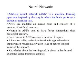
1. Neural Networks • Artificial neural network (ANN) is a machine learning approach inspired by the way in which the brain performs a particular learning task. • ANNs are modeled on human brain and consists of a number of artificial neurons. • Neuron in ANNs tend to have fewer connections than biological neurons. • Each neuron in ANN receives a number of inputs. • A function called activation function is applied to these inputs which results in activation level of neuron (output value of the neuron). • Knowledge about the learning task is given in the form of examples called training examples.

2. An Artificial Neural Network is specified by: • neuronmodel: the information processing unit of the NN, • an architecture: a set of neurons and links connecting neurons. Each link has a weight, • a learning algorithm: used for training the NN by modifying the weights in order to model a particular learning task correctly on the training examples. • The aim is to obtain a NN that generalizes well, i.e., that behaves correctly on new instances of the learning task.

3. The Neuron • The neuron is the basic information processing unit of a NN. It consists of: • A set of links, describing the neuron inputs, with weightsW1, W2, …, Wm • An adder function (linear combiner) for computing the weighted sum of the inputs: (real numbers) • Activation function for limiting the amplitude of the neuron output. Here ‘b’ denotes bias.

4. Bias b x1 w1 Activation function Local Field v Output y Input values x2 w2 Summing function xm wm weights The Neuron diagram

5. Bias of a Neuron • The bias b has the effect of applying an transformation to the weighted sum u v = u + b • The bias is an external parameter of the neuron. It can be modeled by adding an extra input. • vis called induced field of the neuron

6. Neuron Models • The choice of activation function determines the neuron model. Examples: • step function: • ramp function: • sigmoid function with z,x,y parameters • Gaussian function:

7. Network architectures • Three different classes of network architectures • single-layer feed-forward • multi-layer feed-forward • recurrent • The architecture of a neural network is linked with the learning algorithm used to train

8. Single Layer Feed-forward Input layer of source nodes Output layer of neurons

9. b (bias) x1 w1 v y x2 w2 (v) wn xn Perceptron: Neuron Model(Special form of single layer feed forward) • The perceptron was first proposed by Rosenblatt (1958) is a simple neuron that is used to classify its input into one of two categories. • A perceptron uses a step function that returns +1 if weighted sum of its input is greater than equal to a threshold  and -1 otherwise

10. Perceptron for Classification • The perceptron is used for binary classification. • How can we train a perceptron for a classification task? • We try to find suitable values for the weights in such a way that the training examples are correctly classified. • Geometrically, we try to find a hyper-plane that separates the examples of the two classes. • The perceptron can only model linearly separable classes. • When the two classes are not linearly separable, it may be desirable to obtain a linear separator that minimizes the mean squared error. • Given training examples of classes C1, C2 train the perceptron in such a way that : • If the output of the perceptron is +1 then the input is assigned to class C1 • If the output is -1 then the input is assigned to C2

11. Learning Process for perceptron • Initially assign random weights to input between -0.5 and +0.5 • Training data is presented to perceptron and its output is observed. • If output is incorrect, the weights are adjusted accordingly using following formula. • wi wi + (a* xi *e), • where e is error produced and ‘a’ is learning rate (0  a  1) • ‘a’ is defined as 0 if output is correct, it is +ve if output is too low and –ve if output is too high. • Once the modification to weights has taken place, the next piece of training data is used in the same way. • Once all the training data have been applied, the process starts again until all the weights are correct and all errors are zero. • Each iteration of this process is known as an epoch.

12. Example: Perceptron to learn OR function • Initially consider w1 = -0.2 and w2 = 0.4 • Training data say, x1 = 0 and x2 = 0. Expected output is 0. • Compute y = Step(w1*x1 + w2*x2) = 0. Output is correct so weights are not changed. • For training data x1=0 and x2 = 1, output is 1 • Compute y = Step(w1*x1 + w2*x2) = 0.4 = 1. Output is correct so weights are not changed. • Next training data x1=1 and x2 = 0 and output is 1 • Compute y = Step(w1*x1 + w2*x2) = - 0.2 = 0. Output is incorrect, hence weights are changed. • Assume a = 0.2 and error e=1 • wi = wi + (a * xi * e) gives w1 = 0 and w2 =0.4 • Repeat the process till we get stable result.

13. Perceptron: Limitations • The perceptron can only model linearly separable functions, (those can be drawn in 2-dim graph and single straight line separating values in two part )such as the following boolean functions: • AND • OR • COMPLEMENT • It cannot model the XOR (non linearly separable). • When the two classes are not linearly separable, it may be desirable to obtain a linear separator that minimizes the mean squared error.

14. Multi layer feed-forward 3-4-2 Network Output layer Input layer Hidden Layer

15. Multi layer feed-forward NN (FFNN) • FFNN is a more general network architecture. • Between the input and output layers, there are hidden layers, as illustrated below. • Hidden nodes do not directly receive inputs nor send outputs to the external • environment. • FFNNs overcome the limitation of single-layer NN: they can handle non-linearly separable learning tasks. Input layer Output layer Hidden Layer

16. XOR problem • A typical example of non-linearly separable function is the XOR. This function takes two input arguments with values in {-1,1} and returns one output in {-1,1}, as specified in the following table: • Here -1 and 1 are encoding of the truth values false and true, • Respectively and XOR computes the logical exclusive or, which yields • true if and only if the two inputs have different • truth values.

17. x1 1 -1 1 x2 -1 XOR problem • In this graph of the XOR, input pairs giving output equal to 1 and -1 are depicted with green and red circles, respectively. • These two classes (green and black) cannot be separated using a line. We have to use two lines, like those depicted in blue.

18. -1 0.1 +1 +1 -1 -1 +1 +1 XOR problem • The following NN with two hidden nodes realizes this non-linear separation, where each hidden node describes one of the two blue lines. • This NN uses the sign activation function. Arrows from input nodes to two hidden nodes indicate the directions of the weight vectors (1,-1) and (-1,1). • They indicate the regions where the network output will be 1. • The output node is used to combine the outputs of the two hidden nodes. x1 x2 -1

19. FFNN NEURON MODEL • The classical learning algorithm of FFNN is based on the gradient descent method. For this reason the activation function used in FFNN are continuous functions of the weights, differentiable everywhere. • A typical activation function that can be viewed as a continuous approximation of the step (threshold) function is the Sigmoid Function. The activation function for node j is:

20. 1 Increasing a -10 -8 -6 -4 -2 2 4 6 8 10 FFNN NEURON MODEL when ‘a’ tends to infinity then  becomes the step function

21. Training Algorithm: Backpropagation • The Backpropagation algorithm learns in the same way as single perceptron. • It searches for weight values that minimize the total error of the network over the set of training examples (training set). • Backprop consists of the repeated application of the following two passes: • Forward pass: in this step the network is activated on one example and the error of (each neuron of) the output layer is computed. • Backward pass:in this step the network error is used for updating the weights (credit assignment problem). Start at the output layer, the error is propagated backwards through the network layer by layer. This is done by recursively computing the local gradient of each neuron.

22. Backprop algorithm – Contd. • Consider a network of three layers. Let us use i to represent nodes in input layer, j to represent nodes in hidden layer and k represent nodes in output layer. • wij refers to weight of connection between a node in input layer and node in hidden layer. • The following equation is used to derive the output value Yj of node j • threshold for node j • Xj =  xi . wij - j , 1 i  nthe number of inputs to node j,

23. Total Mean Squared Error • The error of output neuron k after the activation of the network on the n-th training example (x(n), d(n)) is: ek(n) = dk(n) – yk(n) • The network error is the sum of the squared errors of the output neurons: • The total mean squared error is the average of the network errors of the training examples.

24. Weight Update Rule • The Backprop weight update rule is based on the gradient • descent method: • It takes a step in the direction yielding the maximum decrease of the network error E. • This direction is the opposite of the gradient of E. • Iteration of the Backprop algorithm is usually terminated when the sum of squares of errors of the output values for all training data in an epoch is less than some threshold such as 0.01

25. Backprop • Back-propagation training algorithm • Backprop adjusts the weights of the NN in order to minimize the network total mean squared error. Network activation Forward Step Error propagation Backward Step

26. Error backpropagation The flow-graph below illustrates how errors are back-propagated to hidden neuron j w1j e1 ’(v1) 1 j ’(vj) wkj ek ’(vk) k wm j em m ’(vm)

27. Backprop learning algorithm(incremental-mode) n=1; initializew(n) randomly; while (stopping criterion not satisfied or n <max_iterations) for each example (x,d) - run the network with input x and compute the output y - update the weights in backward order starting from those of the output layer: with computed using the (generalized) Delta rule end-for n = n+1; end-while;

28. Backprop algorithm • In the batch-mode the weights are updated only after all examples have been processed, using the formula • The learning process continues until the stopping condition is satisfied. • In the incremental mode choose a randomized ordering for selecting the examples in the training set in order to avoid poor performance.

29. Stopping criterions • Sensible stopping criterions: • total mean squared error change: Back-prop is considered to have converged when the absolute rate of change in the average squared error per epoch is sufficiently small (in the range [0.1, 0.01]). • generalization based criterion: After each epoch the NN is tested for generalization. If the generalization performance is adequate then stop. If this stopping criterion is used then the part of the training set used for testing the network generalization will not used for updating the weights.

30. Applicability of FFNN Boolean functions: • Every boolean function can be represented by a network with a single hidden layer Continuous functions: • Every bounded piece-wise continuous function can be approximated with arbitrarily small error by a network with one hidden layer. • Any continuous function can be approximated to arbitrary accuracy by a network with two hidden layers.

31. Applications of FFNN Classification, pattern recognition: • FFNN can be applied to tackle non-linearly separable learning problems. • Recognizing printed or handwritten characters, • Face recognition • Classification of loan applications into credit-worthy and non-credit-worthy groups • Analysis of sonar radar to determine the nature of the source of a signal Regression and forecasting: • FFNN can be applied to learn non-linear functions (regression) and in particular functions whose inputs is a sequence of measurements over time (time series).

32. Recurrent network • Feed forward network is acyclic ( no cycle) as data passes from input to the output nodes and not vice versa. • Once the FFNN is trained, its state is fixed and does not alter as new data is presented to it. It does not have memory. • A recurrent network can have connections that go backward from output to input nodes . • In this way , a recurrent network’s internal state can alter as sets of input data are presented. It can be said to have memory. • Useful in solving problems where the solution depends not just on the current inputs but on all previous inputs. (predict stock market price, weather forecast). • When learning, a recurrent network feeds its inputs through the network, including feeding data back from outputs to inputs an repeats this process until the values of the outputs do not change. • This state is called equilibrium or stability.

33. d d d Recurrent network Recurrent Network with hidden neuron: unit delay operator d is used to model a dynamic system input hidden output

34. A recurrent network can have connections that go backward from output nodes to input nodes and in fact can have arbitrary connections between any nodes. • While learning, the recurrent network feeds its inputs through the network including feeding data back from outputs to inputs and repeat this process until the values of the outputs do not change. • Such point is called a state of equilibrium or stability. • Useful applications to predict • stock market, • weather etc.

35. NN DESIGN • Data representation • Network Topology • Network Parameters • Training • Validation

36. Data Representation • Data representation depends on the problem. In general ANNs work on continuous (real valued) attributes. Therefore symbolic attributes are encoded into continuous ones. • Attributes of different types may have different ranges of values which affect the training process. Normalization may be used, like the following one which scales each attribute to assume values between 0 and 1. for each value of attribute , where are the minimum and maximum value of that attribute over the training set.

37. Network Topology • The number of layers and of neurons depend on the specific task. In practice this issue is solved by trial and error. • Two types of adaptive algorithms can be used: • start from a large network and successively remove some neurons and links until network performance degrades. • begin with a small network and introduce new neurons until performance is satisfactory.

38. Network parameters • How are the weights initialized? • How is the learning rate chosen? • How many hidden layers and how many neurons? • How many examples in the training set?

39. Initialization of weights • In general, initial weights are randomly chosen, with typical values between -1.0 and 1.0 or -0.5 and 0.5. • If some inputs are much larger than others, random initialization may bias the network to give much more importance to larger inputs. In such a case, weights can be initialized as follows: For weights from the input to the first layer For weights from the first to the second layer

40. Choice of learning rate • The right value of depends on the application. Values between 0.1 and 0.9 have been used in many applications. • Other heuristics adapt  during the training as described in previous slides.

41. Training • Rule of thumb: • the number of training examples should be at least five to ten times the number of weights of the network. • Other rule: |W|= number of weights a=expected accuracy on test set

42. Radial-Basis Function Networks • A function is radial basis(RBF) if its output depends on (is a non-increasing function of) the distance of the input from a given stored vector. • RBFs represent local receptors, as illustrated below, where each green point is a stored vector used in one RBF. • In a RBF network one hidden layer uses neurons with RBF activation functions describing local receptors. Then one outputnode is used to combine linearly the outputs of the hidden neurons. w3 The output of the red vector is “interpolated” using the three green vectors, where each vector gives a contribution that depends on its weight and on its distance from the red point. In the picture we have w2 w1

43. x1 w1 x2 y wm1 xm RBF ARCHITECTURE • One hidden layer with RBF activation functions • Output layer with linear activation function.

44. HIDDEN NEURON MODEL • Hidden units: use radial basis functions the output depends on the distance of the input x from the center t φ( || x - t||) x1 φ( || x - t||) t is called center  is called spread center and spread are parameters x2 xm

45. Hidden Neurons • A hidden neuron is more sensitive to data points near its center. • For Gaussian RBF this sensitivity may be tuned by adjusting the spread , where a larger spread impliesless sensitivity. • Biological example: cochlear stereocilia cells (in our ears ...) have locally tuned frequency responses.

46. center Small  Large  Gaussian RBF φ φ :  is a measure of how spread the curve is:

47. Types of φ • Multiquadrics: • Inversemultiquadrics: • Gaussianfunctions (most used):

48. x2 (0,1) (1,1) 0 1 y x1 (0,0) (1,0) Example: the XOR problem • Input space: • Output space: • Construct an RBF pattern classifier such that: (0,0) and (1,1) are mapped to 0, class C1 (1,0) and (0,1) are mapped to 1, class C2

49. φ2 (0,0) Decision boundary 1.0 0.5 (1,1) 1.0 φ1 0.5 (0,1) and (1,0) Example: the XOR problem • In the feature (hidden layer) space: • When mapped into the feature space < 1 , 2 > (hidden layer), C1 and C2become linearly separable. Soa linear classifier with 1(x) and 2(x) as inputs can be used to solve the XOR problem.

50. x1 t1 -1 y x2 t2 -1 +1 RBF NN for the XOR problem