Multi-Layer Perceptron (MLP)
Multi-Layer Perceptron (MLP). Neural Networks Lectures 5+6. x 1. x n. Today we will introduce the MLP and the backpropagation algorithm which is used to train it MLP used to describe any general feedforward (no recurrent connections) network


Multi-Layer Perceptron (MLP)
E N D
Presentation Transcript
Multi-Layer Perceptron (MLP) Neural Networks Lectures 5+6
x1 xn Today we will introduce the MLP and the backpropagation algorithm which is used to train it MLP used to describe any general feedforward (no recurrent connections) network However, we will concentrate on nets with units arranged in layers
x1 xn NB different books refer to the above as either 4 layer (no. of layers of neurons) or 3 layer (no. of layers of adaptive weights). We will follow the latter convention 1st question: what do the extra layers gain you? Start with looking at what a single layer can’t do
XOR problem Single layer generates a linear decision boundary XOR (exclusive OR) problem 0+0=0 1+1=2=0 mod 2 1+0=1 0+1=1 Perceptron does not work here
+1 Minsky & Papert (1969) offered solution to XOR problem by combining perceptron unit responses using a second layer of units +1 1 3 2
(1,-1) (1,1) (-1,-1) (-1,1) This is a linearly separable problem! Since for 4 points { (-1,1), (-1,-1), (1,1),(1,-1) } it is always linearly separable if we want to have three points in a class
Three-layer networks x1 x2 Input Output xn Hidden layers
Properties of architecture • No connections within a layer Each unit is a perceptron
Properties of architecture • No connections within a layer • No direct connections between input and output layers Each unit is a perceptron
Properties of architecture • No connections within a layer • No direct connections between input and output layers • Fully connected between layers Each unit is a perceptron
Properties of architecture • No connections within a layer • No direct connections between input and output layers • Fully connected between layers • Often more than 3 layers • Number of output units need not equal number of input units • Number of hidden units per layer can be more or less than • input or output units Each unit is a perceptron Often include bias as an extra weight
What do each of the layers do? 3rd layer can generate arbitrarily complex boundaries 1st layer draws linear boundaries 2nd layer combines the boundaries
Can also view 2nd layer as using local knowledge while 3rd layer does global With sigmoidal activation functions can show that a 3 layer net can approximate any function to arbitrary accuracy: property of Universal Approximation Proof by thinking of superposition of sigmoids Not practically useful as need arbitrarily large number of units but more of an existence proof For a 2 layer net, same is true for a 2 layer net providing function is continuous and from one finite dimensional space to another
BP gradient descent method + multilayer networks
In the perceptron/single layer nets, we used gradient descent on the error function to find the correct weights: D wji = (tj - yj) xi We see that errors/updates are local to the node ie the change in the weight from node i to output j (wji) is controlled by the input that travels along the connection and the error signal from output j x1 (tj - yj) x1 ? x2 • But with more layers how are the weights for the first 2 layers found when the error is computed for layer 3 only? • There is no direct error signal for the first layers!!!!!
Credit assignment problem • Problem of assigning ‘credit’ or ‘blame’ to individual elements • involved in forming overall response of a learning system • (hidden units) • In neural networks, problem relates to deciding which weights • should be altered, by how much and in which direction. • Analogous to deciding how much a weight in the early layer contributes to the output and thus the error • We therefore want to find out how weight wij affects the error ie we want:
Backpropagation learning algorithm ‘BP’ Solution to credit assignment problem in MLP Rumelhart, Hinton and Williams (1986) BP has two phases: Forward pass phase: computes ‘functional signal’, feedforward propagation of input pattern signals through network
Backpropagation learning algorithm ‘BP’ Solution to credit assignment problem in MLP. Rumelhart, Hinton and Williams (1986) (though actually invented earlier in a PhD thesis relating to economics) BP has two phases: Forward pass phase: computes ‘functional signal’, feedforward propagation of input pattern signals through network Backward pass phase: computes ‘error signal’, propagates the error backwards through network starting at output units (where the error is the difference between actual and desired output values)
Two-layer networks Outputs of 1st layer zi x1 x2 y1 Inputs xi Outputs yj ym 2nd layer weights wij from j to i xn 1st layer weights vij from j to i
We will concentrate on three-layer, but could easily generalize to more layers zi (t) = g( Sj vij (t)xj (t) ) at time t = g ( ui (t) ) yi (t) = g( Sj wij (t)zj (t) ) at time t = g ( ai (t) ) a/u known as activation, g the activation function biases set as extra weights
Forward pass Weights are fixed during forward and backward pass at time t 1. Compute values for hidden units 2. compute values for output units yk wkj(t) zj vji(t) xi
Backward Pass Will use a sum of squares error measure. For each training pattern we have: where dk is the target value for dimension k. We want to know how to modify weights in order to decrease E. Use gradient descent ie both for hidden units and output units
The partial derivative can be rewritten as product of two terms using chain rule for partial differentiation both for hidden units and output units How error for pattern changes as function of change in network input to unit j Term A How net input to unit j changes as a function of change in weight w Term B
Term B first: Term A Let (error terms). Can evaluate these by chain rule:
Backward Pass wki wji Dk Dj Weights here can be viewed as providing degree of ‘credit’ or ‘blame’ to hidden units di di = g’(ai) Sj wji Dj
Combining A+B gives So to achieve gradient descent in E should change weights by vij(t+1)-vij(t) = h d i (t) xj (n) wij(t+1)-wij(t) = h D i (t) zj (t) Where h is the learning rate parameter (0 < h <=1)
Summary Weight updates are local output unit hidden unit
5 Multi-Layer Perceptron (2) -Dynamics of MLP Topic Summary of BP algorithm Network training Dynamics of BP learning Regularization
Algorithm (sequential) 1. Apply an input vector and calculate all activations, a and u 2. Evaluate Dk for all output units via: (Note similarity to perceptron learning algorithm) 3. Backpropagate Dks to get error terms d for hidden layers using: 4. Evaluate changes using:
v10= 1 v20= 1 Once weight changes are computed for all units, weights are updated at the same time (bias included as weights here). An example: v11= -1 x1 w11= 1 y1 v21= 0 w21= -1 v12= 0 w12= 0 x2 y2 v22= 1 w22= 1 Use identity activation function (ie g(a) = a)
All biases set to 1. Will not draw them for clarity. Learning rate h = 0.1 v11= -1 x1 x1= 0 w11= 1 y1 v21= 0 w21= -1 v12= 0 w12= 0 x2 x2= 1 y2 v22= 1 w22= 1 Have input [0 1] with target [1 0].
Forward pass. Calculate 1st layer activations: u1 = 1 v11= -1 x1 w11= 1 y1 v21= 0 w21= -1 v12= 0 w12= 0 x2 y2 v22= 1 w22= 1 u2 = 2 u1 = -1x0 + 0x1 +1 = 1 u2 = 0x0 + 1x1 +1 = 2
Calculate first layer outputs by passing activations thru activation functions z1 = 1 v11= -1 x1 w11= 1 y1 v21= 0 w21= -1 v12= 0 w12= 0 x2 y2 v22= 1 w22= 1 z2 = 2 z1 = g(u1) = 1 z2 = g(u2) = 2
Calculate 2nd layer outputs (weighted sum thru activation functions): v11= -1 x1 w11= 1 y1= 2 v21= 0 w21= -1 v12= 0 w12= 0 x2 y2= 2 v22= 1 w22= 1 y1 = a1 = 1x1 + 0x2 +1 = 2 y2 = a2 = -1x1 + 1x2 +1 = 2
Backward pass: v11= -1 x1 w11= 1 D1= -1 v21= 0 w21= -1 v12= 0 w12= 0 x2 D2= -2 v22= 1 w22= 1 Target =[1, 0] so d1 = 1 and d2 = 0 So: D1 = (d1 - y1 )= 1 – 2 = -1 D2 = (d2 - y2 )= 0 – 2 = -2
Calculate weight changes for 1st layer (cf perceptron learning): z1 = 1 v11= -1 D1 z1 =-1 x1 w11= 1 v21= 0 w21= -1 D1 z2 =-2 v12= 0 w12= 0 D2 z1 =-2 x2 v22= 1 w22= 1 D2 z2 =-4 z2 = 2
Weight changes will be: v11= -1 x1 w11= 0.9 v21= 0 w21= -1.2 v12= 0 w12= -0.2 x2 v22= 1 w22= 0.6
But first must calculate d’s: v11= -1 x1 D1 w11= -1 D1= -1 v21= 0 D2 w21= 2 v12= 0 D1 w12= 0 x2 D2= -2 v22= 1 D2 w22= -2
D’s propagate back: d1= 1 v11= -1 x1 D1= -1 v21= 0 v12= 0 x2 D2= -2 v22= 1 d2 = -2 d1 = - 1 + 2 = 1 d2 = 0 – 2 = -2
And are multiplied by inputs: d1 x1 = 0 v11= -1 x1= 0 D1= -1 v21= 0 d1 x2 = 1 v12= 0 d2 x1 = 0 x2= 1 D2= -2 v22= 1 d2 x2 = -2
Finally change weights: v11= -1 x1= 0 w11= 0.9 v21= 0 w21= -1.2 v12= 0.1 w12= -0.2 x2= 1 v22= 0.8 w22= 0.6 Note that the weights multiplied by the zero input are unchanged as they do not contribute to the error We have also changed biases (not shown)
Now go forward again (would normally use a new input vector): z1 = 1.2 v11= -1 x1= 0 w11= 0.9 v21= 0 w21= -1.2 v12= 0.1 w12= -0.2 x2= 1 v22= 0.8 w22= 0.6 z2 = 1.6
Now go forward again (would normally use a new input vector): v11= -1 x1= 0 y1 = 1.66 w11= 0.9 v21= 0 w21= -1.2 v12= 0.1 w12= -0.2 x2= 1 v22= 0.8 w22= 0.6 y2 = 0.32 Outputs now closer to target value [1, 0]
Activation Functions How does the activation function affect the changes? Where: - we need to compute the derivative of activation function g - to find derivative the activation function must be smooth (differentiable)
Sigmoidal (logistic) function-common in MLP where k is a positive constant. The sigmoidal function gives a value in range of 0 to 1. Alternatively can use tanh(ka) which is same shape but in range –1 to 1. Input-output function of a neuron (rate coding assumption) Note: when net = 0, f = 0.5
Derivative of sigmoidal function is Derivative of sigmoidal function has max at a = 0., is symmetric about this point falling to zero as sigmoid approaches extreme values
Since degree of weight change is proportional to derivative of activation function, weight changes will be greatest when units receives mid-range functional signal and 0 (or very small) extremes. This means that by saturating a neuron (making the activation large) the weight can be forced to be static. Can be a very useful property
Summary of (sequential) BP learning algorithm Set learning rate Set initial weight values (incl. biases): w, v Loop until stopping criteria satisfied: present input pattern to input units compute functional signal for hidden units compute functional signal for output units present Target response to output units computer error signal for output units compute error signal for hidden units update all weights at same time increment n to n+1 and select next input and target end loop