Download
1 / 25
250 likes | 508 Views
OSI SAF VIIRS Cloud Mask L. Lavanant S. Péré, H. Le Gléau Météo-France/CMS. MAIA development context. MAIA-v1 1998 & MAIA-v2 2000 : to document NOAA HIRS sounder footprint from collocated AVHRR in AAPP package MAIA-v3 2002 - … AVHRR full resolution.

E N D
OSI SAF VIIRS Cloud Mask L. Lavanant S. Péré, H. Le Gléau Météo-France/CMS
MAIA development context MAIA-v11998 & MAIA-v2 2000 : to document NOAA HIRS sounder footprint from collocated AVHRR in AAPP package MAIA-v32002-… AVHRR full resolution. CMSoperationalprocessing of NOAA and METOP for OSI SAF SST production and other applications (images for MF Immediate forecasting, AAPP) Based on NWC SAF v1.2 scientific characteristics MAIA-v4 2012 VIRRS and AVHRR full resolution. CMS pre-operational processing of VIIRS for SST production,.. Based on: NWC SAF v2010 for most of the scheme: dynamic thresholds, tests (i.e. sea ice/snow detection,..., texture), … MODIS ATBD & VIIRS OAD for confidence level, cloud phase, tests with new channels
Content VIIRS instrument and used channels in MAIA SEVIRI VIIRS(NPP/JPSS)AVHRR Pixel size(sub-point /nadir) 3km M:750m /I:375m1.1km Channel Sensitivity Central Wavelengthμm Filters Width M1 VIS 04 A0.410.40-0.42 M4 VIS 05 Cc+A 0.490.48-0.50 M5 / I1 VIS 06 Cc+Ct+Cm+A+V 0.65 0.67/0.640.630.56-0.71 0.66-0.680.58-0.68 M7 / I2 VIS 08 Cc+Ct +Cm+A+V0.81 0.87/0.860.860.74-0.880.85-0.880.72-1.00 M9 NIR 13 Cirrus+Cc+A1.3751.37-1.38 M10 NIR 16 Snow+Cc+Ct+A 1.641.611.611.50-1.781.58-1.641.58-1.64 M11 NIR 22 Cm + A2.252.22-2.27 M12 / I4 IR 37 Cc+Ct+Ts+D+F 3.903.75/3.743.743.48-4.363.66-3.843.55-3.93 M13 IR 40 Ts+D+F 4.053.97-4.13 M14 IR 87 Cm8.708.558.30-9.10 8.4-8.7 M15 / I5 IR 108 Cc+Ts +D+F10.810.75/11.4510.89.80-11.810.26-11.2610.3-11.3 M16 IR 120Cc+Ct+Ts+D12.012.012.011.0-13.011.54-12.4911.5-12.5 Cc: Cloud cover / Ct: Cloud type / Cm: Cloud microphysic / A: Aerosol / D:Dust, Ash / F:Fire / V: Vegetation 3
Content MAIA-v4 VIIRS overview HDF5 input VIIRS observations 12 Medium channels Local texture from 4 Imaging channels or M neighbors position viewing & solar angles Forecast: detection: T2m, TWVC, Ps type: T500, 700, 850hPa Pc: T,q on 51 RTTOV levels HDF5 output Position & geometry clear/cloud/snow flag & confidence level Cloud type Cloud pressure Cloud phase SST • On pixels: • cloud detection • SST for clear, marine • cloud type • cloud pressure • cloud phase On small cells: • Bg conditions • In-line thresholds values • SST_min atlas • 0.6mm Refl._max atlas • Land type atlas • Surface elevation atlas Look-up thresholds tables • OSI SAF SST coefficients • SST_moy atlas RTTOVv9.3 & 6S off-line simulations depending on satellite 4
Multi-spectral threshold approach applied to each pixel of the granule (global or direct readout) First test : snow/sea-ice (daytime). If successful, the pixel considered clear. Otherwise, apply a sequence of tests for the identification of cloudy pixels with: spectral features (single channels, ratios, differences) depending on surface type (sea/land/coast/desert/perm. snow) solar illumination (daytime/night/twilight/sunglint) local spatial texture in the M footprints using the 350m I channels or using M neighbors dynamic thresholds, except for local texture and SST test (4K threshold) Thresholds determined in-line at a 0.1°x 0.1° resolution: Thermal bands: interpolation in look-uptables using the TWVC forecast & viewing angle. The choice of tables depends on surface type, illumination, zenith angle, Ts (clim or forecast) Visible bands: simulation of the TOA reflectance with: surface reflectance from clim. (land) or model: Cox&Munk (ocean), LeRoux (snow) interpolation in look-up tables to estimate the atmospheric absorption Polynomial regressions function of the azimuth angle Content Cloud detection description (1) 5
Confidence level (similar to MODIS ATBD/VIIRS AOD) : individual confident value for all tests of a sequence, based on proximity to the confident clear and confident cloudy threshold values the tests are groupedto getfive group confident value from the individual values Four final confidentlevels using the confident values of the groups: confident_clear / probably_clear / probably_cloudy / confident_cloudy Quality level Each channel/pixel is appended with a quality flag to allow/discard a channel during the test serie from (number of tests passed /maximum number of tests in a test serie) 0=high (all tests done) / 1=medium (>50% done) / 2=poor (<50% done) / 3=bad (no test done) SST product For confident_clear marine pixels, computes the SST using the OSI SAF models & Mean_SST climatogoly Content Cloud detection description (2) 6
Content cloud detection tests used in daytime 7
For each probably_cloudy and confident_cloudy pixel, ten cloud categories: five opaque clouds according to their altitude, three semi-transparent classes according to their thickness, one class of semi-transparent clouds above lower clouds, one fractional clouds class Apply a sequence of spectral and texture tests. Based on spectral features (10.8mm–12.0mm, 3.7mm–10.8mm, 0.6mm) and local spatial texture (10.8mm,0.6mm), cloud are separated into two sets: fractional and high semi-transparent clouds, separated using 8.7mm–10.8mm low/medium/high opaque clouds, separated using 10.8mm - forecast air temperatures In-line thesholds for : IR channel differences: from interpolation in look-up tables using the TWVC forecast & viewing angle 10.8mm test: function of the forecast air temperatures at 850, 700, 500 hPa pressure levels visible tests: look-up tables empirically derived using a training dataset Content Cloud classification description 8
Cloud pressure For probably_cloudy and confident_cloudy pixels contaminated with opaque clouds: A cloud top temperature is determined from 10.8mm and a correcting value to account for the atmosphere above. correcting value from interpolation in a look-up table function of viewing angle & 10.8mm Verifies that the vertical forecast air temperature profile is associated with temperature inversion/subsidence Provides a cloud top pressure using the vertical air temperature profile Cloud phase For VIIRS, for confident_cloudy pixels, characterisation in 5 cloud phases: Water Cloud, Mixed Phase Cloud, Opaque Ice Cloud, Cirrus Non-Opaque Cloud, Cloud Overlap Following the reference paper Pavolonis, M. J., A. K. Heidinger and T. Uttal: Daytime Global Cloud Typing from AVHRR and VIIRS: Algorithm Description, Validation,and Comparisons. Journal of Applied Meteorology, 2005. Content Cloud pressure and phase description 9
SSTclimatologies: global and twice-monthly datasets resolution: 0.05*0.05 degrees. In C*100 based on NOAA-AVHRR imagery (Faugère et al, 2001) 2 separated climatologies: minimum of SST on the grid for the cloud detection mean SST on the grid for the SST calculation of the confident_clear marine pixels 24 HDF5 files of 50MB each organized by latitude bands of 10 degrees Visible reflectance ( 0.659mm band) climatology (%*100): global and about twice-monthly datasets resolution: 0.05*0.05 degrees based on MODIS black-sky albedo maps of one minute resolution. corrected to 20% over snow area 23 HDF5 files of 50MB each organized by latitude bands of 10 degrees Surface type & elevation files : HDF5 files at a 0.02*0.02 degrees resolution, organized by latitude bands of 10 degrees Surface type atlas (sea / land / desert / snow_always / coast) from GTOPO30 Elevation atlas from MODIS MOD12Q1 global land cover Content Ancillary datasets (1) 10
Look-up tables: Satellite-dependant derived off-line: Thermal bands: RTTOV-v9, ECMWF climatological profiles database (Chevallier, 2001) 5 secant angles, 7 skin-air surface temperatures Sets of surface emissivities (Masuda over sea/Salisbury and D’Aria over land) Visible channels: 6S, a maritime (sea) and continental (land) aerosol of 70km horizontal visibility, a wide range of angles, water vapor and ozone content Forecast: The two forecast files surrounding the observation are read in GRIB format (ECMWF or Arpège allowed by the script). Mandatory fields: geometric altitude, surface pressure, skin and air surface temperatures and forecast profile (T, q) on atmospheric levels. Time interpolation for the T, Ps parameters at the observation acquisition Spatial interpolation for all parameters at the observation position Vertical interpolation for the surface pressure at the observation altitude Vertical interpolation/extrapolation on the 51 RTTOV levels Content Ancillary datasets (2) 11
Validation efforts • First VIIRS cloud mask outputs in march 2012. • First evaluation of all products during the first months. Comparison to: • NWC SAF SEVIRI cloud classification • MODIS confidence and cloud phase • NWP SST for marine confident_clear data • Targets collection over Europe/North Africa • Daily monitoring by nephanalyst / experienced persons • Systematic selection of bad classified data • To tune the thresholds and improve the tests sequences • CMS/MAIA and SMHI/PPS inter-comparison on common acquisitions • related to OSI SAF validation WP • Comparison to Caliop products
Unprocessed Cloudfree land Cloudfree sea Snow covere Sea ice Very low clouds Low clouds Medium level clouds High clouds Very high clouds Very thin cirrus Thin cirrus Thick cirrus Cirrus above low/medium Fractional clouds Unclassified First evaluations of the VIIRS cloud mask Comparisons to SAFNWC SEVIRI cloud type VIIRS. 11h26 – 14h48 SEVIRI. 12h15 Example of VIIRS and time-nearest NWC SAF SEVIRI classification over France on 2012-03-22. The different spatial resolution of the two instruments (VIIRS:~750m and SEVIRI: ~4-5kms) has an impact in the characterization of fractional clouds. SEVIRI detects more thin semi-transparent clouds in edge of clouds.
First evaluations of the VIIRS cloud mask Comparison of VIIRS and SEVIRI clear and cloud classification on homogeneous matchups Matchups with: • less than 7 minutes between VIIRS and SEVIRI acquisitions, • an homogeneous classification in a • local 3x3 pixels box around the matchup for SEVIRI • local 0.1°x 0.1° box for VIIRS(to avoid problems with the complex navigation of VIIRS). The coherence in clear detection is very good. The main disagreement concerns the semi-transparent clouds. Agreement in % for each cloud class category
First evaluations of the VIIRS cloud mask Confident cloudy Probably cloudy Probably clear Confident clear Comparisons to MODIS MYD35 cloud confidence MODIS. 11h40 – 15h00 VIIRS. 11h26 – 14h48 VIRRS and MODIS MYD35 cloud confidence for the 3 successive passes of 2012-03-12. The time departure between VIIRS and MODIS is about 15mn. The main differences concern the ‘probably clear’ class, due to the distance to the thresholds, the different tests,..
First evaluations: Comparison in cloud fraction MAIA VIIRS – MODIS MYD35 To reduce the problem of the difference in pixel size and navigation of the instruments, cloud amounts are computed in 0.5 degree cells on the CMS direct readout acquisition area for VIIRS, SEVIRI and MODIS. Over sea, VIIRS cloud fractions are slightly smaller than for SEVIRI, probably due to sub-clouds in the fov. MAIA VIIRS – NWC SAF SEVIRI
First evaluations: derived Sea Surface Temperatures Comparison of derived SST using the OSI SAF software on the MAIA confident_clear observations to the ECMWF NWP SST analysis fields. The figure shows the distribution of the differences for a 5 day period. Cloud contamination acts to slightly shift the distribution towards negative values.
Targets collection • Targets extraction by visual type evaluation: • PV-Wave visual package • Skilled nephanalyst • Accent on difficult / bad classified data + representative situations • not useful for an un-biased validation • Purpose: improvement of algorithms • Targets data set • 2182 situations selected sofar over Europe (start 3 months ago) • Target: 7*7 scene with all necessary information to re-run the scene • lat, lon, angles, VIIRS Tbs and VIS • forecast, climatologies • Mask outputs , test identification which has declare cloudy • nephanalyse classification • Format: ascii
Targets extracted over Europe Preliminary results No scheme tuning sofar • Targets dataset over Europe: • 2182 targets of 7x7 VIIRS pixels • 3 months of data
Targets extracted over Europe Preliminary results No scheme tuning sofar Night day Observed type of missed clouds VIIRS assigned type of missed clear
Summary • This pre-operational version already works « correctly ». • Slightly less severe than what is necessary for SST production, cloud products also used for imagery…. • Continue the tuning & validation efforts in 2013. • Internal archive of cloud products for the CMS direct broadcast area with name constructed using: • data acquisition type (DB=direct broadcast or GL=global), • date, starting and ending time of the granule, • ascending or descending orbit condition (ASC=ascending, DES=descending), • Day/Night illumination condition(D=day, N=night), • latitude and longitude of the centered pixel in the granule, • orbit number. • Ex: viiCT_npp_DB_20121214_S013613_E013737_DES_N_La068_Lo0018_00001.h5