Download
1 / 35
380 likes | 574 Views
Chapter 2: Statistical Inference. Chapter Outline 2.1 Estimation Confidence Interval Estimates for Population Mean Confidence Interval Estimates for the Difference Between Two Population Mean Confidence Interval Estimates for Population Proportion

E N D
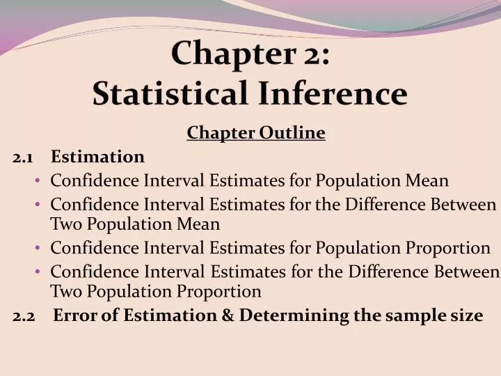
Chapter 2: Statistical Inference Chapter Outline 2.1 Estimation Confidence Interval Estimates for Population Mean Confidence Interval Estimates for the Difference Between Two Population Mean Confidence Interval Estimates for Population Proportion Confidence Interval Estimates for the Difference Between Two Population Proportion 2.2 Error of Estimation & Determining the sample size
Statistical Inference Statistical inference - process of drawing an inference about the data statistically. It concerned in making conclusion about the characteristics of a population based on information contained in a sample. Since populations are characterized by numerical descriptive measures called parameters, therefore, statistical inference is concerned in making inferences about population parameters.
2.1 Estimation In estimation, there are two terms that firstly, should be understand. The two terms involved in estimation are: Estimator :sample statistics used to estimate a population parameter. Estimate: value that obtained from a sample to estimate a population parameter. An estimate of a population parameter may be expressed in two ways: i) Point Estimate ii) Interval Estimate.
Point Estimate A point estimate of a population parameter is a single value of a statistic. For example, the sample mean is a point estimate of the population mean μ. Similarly, the sample proportion is a point estimate of the population proportion P. ii) Interval Estimate An interval estimate is defined by two numbers, between which a population parameter is said to lie. For example, a < μ < b is an interval estimate of the population mean μ. It indicates that the population mean is greater than a but less than b.
Point estimators Choosing the right point estimators to estimate a parameter depends on the properties of the estimators it selves. There are four properties of the estimators that need to be satisfied in which it is considered as best linear unbiased estimators. The properties are: Unbiased Consistent Efficient Sufficient
2.1.1 Confidence Interval Each interval is constructed with regard to a given confidence level and is called a confidence interval. The confidence level associated with a confidence interval states how much confidence we have that this interval contains the true population parameter. The confidence level is denoted by
Example: The brightness of a television picture tube can be evaluated by measuring the amount of current required to achieve a particular brightness level. A random sample of 10 tubes indicated a sample mean microamps and a sample standard deviation is microamps. Find (in microamps) a 99% confidence interval estimate for mean current required to achieve a particular brightness level. Solution: For 99% CI: From t normal distribution table:
Hence 99% CI Thus, we are 99% confident that the mean mean current required to achieve a particular brightness level is between 301.0645 and 333.3355
Exercise: Taking a random sample of 35 individuals waiting to be serviced by the teller, we find that the mean waiting time was 22.0 min and the standard deviation was 8.0 min. Using a 90% confidence estimate the mean waiting time for all individuals waiting in the service line.
ii) Confidence Interval Estimates for the Differences Between Two Population Mean, i) Variance and are known: ii) If the population variances, and are unknown, then the following tables shows the different formulas that may be used depending on the sample sizes and the assumption on the population variances.
Example: Two machines are used to fill plastic bottles with liquid laundry detergent. The standard deviations of fill volume are known to be and fluid ounce for the two machines, respectively. Two random samples of bottles from the machine 1 and bottles from machine 2 are selected, and the sample means fill volume are and fluid ounces. Construct a 90% confidence interval on the mean difference in fill volumes. Interpret the results. Solution: For 90% CI:
We are 90% confidence that the mean difference to fill volumes lies between 1.0163 and 1.1837 fluid ounces.
Example: A study was conducted to compare the starting salaries for university graduates majoring in computer science and engineering. A random sample of 50 recent university graduates in each major were selected and the following information was obtained. Construct a 99% confidence interval for the difference in the mean starting salaries for two majors. Solution: We are 99% confidence that the mean difference of starting salaries for to major lies between -365.6703 and -234.3297.
Exercise: 18 male undergraduate students and 20 female undergraduate students are randomly selected from faculty of mechanical engineering. Result for test 2 SSM 3763 shown the following data: Assume that both population are normally distributed and have equal population variances. Construct a 95% confidence interval for the difference in the two means.
iii) Confidence Interval Estimates for Population Proportion,( )
Example: According to the analysis of Women Magazine in June 2005, “Stress has become a common part of everyday life among working women in Malaysia. The demands of work, family and home place an increasing burden on average Malaysian women”. According to this poll, 40% of working women included in the survey indicated that they had a little amount of time to relax. The poll was based on a randomly selected of 1502 working women aged 30 and above. Construct a 95% confidence interval for the corresponding population proportion. Solution: Let p be the proportion of all working women age 30 and above, who have a limited amount of time to relax, and let be the corresponding sample proportion. From the given information, n = 1502 , = 0.40 , = 1 – 0.40 = 0.60
Hence, 95% CI : Thus, we can state with 95% confidence that the proportion of all working women aged 30 and above who have a limited amount of time to relax is between 37.5% and 42.5%.
Exercise: The wedding ceremony for a couple, Jamie and Robbin will be held in Menara Kuala Lumpur. A survey has been carried out to determine the proportion of people who will come to the ceremony. From 250 invitations, only 180 people agree to attend the ceremony. Find a 90% confidence interval estimate for the proportion of all people who will attend the ceremony.
iv) Confidence Interval Estimates for the Differences Between Two Population Proportion,
Example: Two separate surveys were carried out to investigate whether or not the users of Plus highway were in favour of raising the speed limit on highways. Of the 250 car drivers interviewed, 220 were in favour of raising the speed limit while of the 200 motorists interviewed , 180 were in favour. Find a 95% confidence interval for the difference in proportion between the car drivers and motorist who are in favour of raising the speed limit. Solution: Hence, 95% CI : We are 95% confident that the difference between the car drivers and motorist who are in favour of raising the speed limits lies between -0.0788 and 0.0388.
When we estimate a parameter, all we have is the estimate value from n measurements contained in the sample. There are two questions that usually arise: • How far our estimate will lie from the true value of the parameter? • (ii) How many measurements should be considered in the sample? 2.2 Error of Estimation and Choosing the Sample Size
The distance between an estimate and the estimated parameter is called the error of estimation. For example if most estimates are within 1.96 standard deviations of the true value of the parameter, then we would expect the error of estimation to be less than 1.96 standard deviations of the estimator, with the probability approximately equal to 0.95.
In the process of determining the sample size, we have to define the parameter to be estimated and standard error of its point estimator. • Firstly, choose the bound (B) on the margin of error and confidence coefficient (1-α). • Then, use the following equation to find suitable sample size, n:
Example: The college president asks the statistics teacher to estimate the average age of the students at their college. The statistics teacher would like to be 99% confident that the estimate should be accurate within 1 year. From the previous study, the standard deviation of the ages is known to be 3 years. How large a sample is necessary? Solution:
Example: How large a sample required if we want to be 95% confident that the error in using to estimate p is less than 0.05? If , find the required sample size. Solution:
Exercise: The diameter of a two years old Sentang tree is normally distributed with a Standard deviation of 8 cm. how many trees should be sampled if it is required to estimate the mean diameter within ± 1.5 cm with 95% confidence interval?