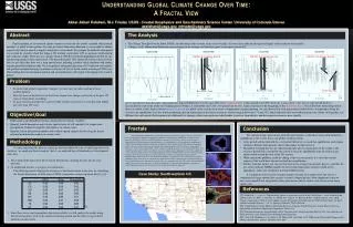
Understanding Global Climate Change Over Time: A Fractal View

1. Understanding Global Climate Change Over Time: A Fractal View Akbar Akbari Esfahani, M.J. Friedel, USGS - Crustal Geophysics and Geochemistry Science Center, University of Colorado Denver aesfahani@usgs.gov, mfriedel@usgs.gov Abstract The Analysis • The Palmer Drought Severity Index (PDSI), an indication of the severity of dry and wet spells. (Lower values indicate drought and higher values indicate wet periods) • Changes in the Information dimension mean changes in the entropy and therefore point to changes in trends.[2] Fractal modeling of reconstructed climate variables revealed that the models coincided with historical anecdotes of global weather patterns. By using the fractal information dimension, it was possible to identify respective dry and wet periods as negative and positive system shocks. For example, the medieval warm period was revealed by a negative shock that began at 950 reaching a peak about 1150, in agreement with historical notes and proxy studies. There also was a positive shock at 1250 that revealed the beginning of the little ice age. Another larger positive shock started about 1750 that peaked about 1930, historically known as the end of the little ice age. Since then there was a steep upward trend, indicating a positive shock coincident with another warming period that continues today. The average Hurst information dimension of 0.75 indicated self-similarity with positive correlated structuring (correlation coefficient of 0.41) of fractal weather over the past 2000 years. These findings have broad economic, political, and social implications with respect to developing water resource policies. Medieval warming period Medieval warming period Medieval warming period Recovery time depends on the length of previous shocks Problem • To understand global temperature changes, we must have an understanding of local weather patterns. • Thus far, most of the forecast for the future temperature changes are based on the past 125 years of temperature recordings. • To gain a historical perspective and to be able to forecast correctly, we need to look further into time than 125 years. Recovery Time Little Ice Age Recovery Time Close to Peak [3] As we can observe from the plots, each region has behaved differently over the past 2000 years. A point shared, is that around year 1000 (40 on the x-axis), there is the start of a dry period which is historically the start of the medieval warming period. Further, at around the year 1250 a wet period can be seen, which correlates to the beginning of the “Little Ice Age.” One of the more interesting aspects that is revealed, is that, there is always a recovery period to a shock to the system, or in terms of temperature and precipitation, we can observe that each dry period is followed by a wet period to bring the system to an equilibrium. It is also worth mentioning that the dimensions of the entire system are closely ranged, between 0.77 and 0.82, which indicates that our weather patterns are closely tied together, yet different for each region. Each region reacts differently to changes, while one region can take decades to recover from shocks, another region can recover more quickly. Objective\Goal • Understand scale-dependent relations among derived climate variables. • Quantify fractal dimension and evaluate spatial nature of self similarity for temperature, precipitation, Palmer Drought Severity Indices in various states. • Quantify fractal information number and evaluate spatial climate shocks using the fractal information dimension number in various states. Fractals Conclusion In the 1960s, Benoît Mandelbrot started investigating self-similarity in papers such as “How Long Is the Coast of Britain?” Statistical Self-Similarity and Fractional Dimension, which built on earlier work by Lewis Fry Richardson. Finally, in 1975 Mandelbrot coined the word "fractal" to denote an object whose Hausdorff–Besicovitch dimension is greater than its topological dimension. He illustrated this mathematical definition with striking computer-constructed visualizations. These images captured the popular imagination; many of them were based on recursion, leading to the popular meaning of the term "fractal". Approximate fractals are easily found in nature. These objects display self-similar structure over an extended, but finite, scale range. Examples include clouds, snow flakes, crystals, mountain ranges, lightning, river networks, cauliflower or broccoli, and systems of blood vessels and pulmonary vessels. Coastlines may be loosely considered fractal in nature. Trees and ferns are fractal in nature and can be modeled on a computer by using a recursive algorithm. This recursive nature is obvious in these examples—a branch from a tree or a frond from a fern is a miniature replica of the whole: not identical, but similar in nature. The connection between fractals and leaves are currently being used to determine how much carbon is contained in trees. In 1999, certain self similar fractal shapes were shown to have a property of "frequency invariance"—the same electromagnetic properties no matter what the frequency. For our models, we use the Fractal information dimension. • The inference that can be drawn from this presentation, is that there seems to be indeed an equilibrium to the system that is our global weather patterns. • A dry period will be followed by a wet period. However, to reach that equilibrium, each region will have different time periods, that it will require for the recovery. • The global warming that we are experiencing right now in certain parts of the world, is the recovery period that is needed by the system to reach its equilibrium from the little ice age, which ended around the turn of the 20th century. • While man made pollution could be adding to the recovery period, it is clear that certain regions of the world have already reached their equilibrium. • Further, from the figures one can see that there exists a long term memory process, and thus the use of just ordinary ARIMA models for forecasting temperature changes would not be appropriate, rather one should use fractional Differencing. • It is important that we relate weather changes not only on a global scale, but also to a temporal scale large enough that can give scientist a bigger picture. More important is that we have to be mindful that our global weather patterns are not on a linear scale but on a non-linear multi-scale. Methodology To truly understand the data set, and to go beyond traditional ways of analyzing data set in statistics, we employed fractal analysis, that is; we analyzed the self similarities of the temporal data, thus, We evaluated the data set for the its fractal Dimensions, splitting the data into 25 year intervals. To understand fractals, we require self-similarities. The following matrix displays the existence of the fractal nature in the data, by calculating the fractal dimensions of 2000 years of PDSI, temperature and precipitation data [1], [4]: [3] Since there are no real temperature data sets available, we will analyze the results using historical anecdotes, such as the medieval warming period and the little ice age to draw inference on the results. Case Study: Southwestern US References [1]: Friedel, M. J. ( in press), Climate change effects on ecosystem services in the United States – issues of national and global security, In: Baba, A., Chambel, A., Friedel, M.J., Haruvy, N., Howard, K.W.F., and Raissouni, B., (eds), 2010, Climate change and its effect on water supplies - Issues of National and Global Security, NATO Science Series, IV. Earth and Environmental Sciences – vol. xx, Springer, Dordrecht, The Netherlands [2]: Daniel Barbara, Chaotic Mining: Knowledge Discovery Using the Fractal Dimension, George Mason University, Information and Software Engineering Department, Fairfax, VA [3]: Plots and data analysis was performed with R, “R-project.com” using the package fdim, by: Fco. Javier Martinez de Pison Ascacibar, et all, Functions for calculating fractal dimension, [4]: Cook, E.R., Woodhouse, C.A., Eakin, C.M., Meko, D.M., and Stahle, D.W. (2004) Long-Term Aridity Changes in the Western United States. Science, 306(5698):1015-1018.