Download
1 / 67
670 likes | 889 Views
Temporal Uncertainty Computation, Fusion, and Visualization in Multisensor Environments. Pramod K. Varshney Kishan G. Mehrotra C. Krishna Mohan Electrical Engineering and Computer Science Dept. Syracuse University Syracuse, NY 13244 Phone: (315) 443-4013 Email: varshney@syr.edu.

E N D
TemporalUncertainty Computation, Fusion, and Visualization in Multisensor Environments Pramod K. Varshney Kishan G. Mehrotra C. Krishna Mohan Electrical Engineering and Computer Science Dept. Syracuse University Syracuse, NY 13244 Phone: (315) 443-4013 Email: varshney@syr.edu
Outline • Introduction • Temporal Update Mechanisms for Decision Making in Probabilistic Networks • Sensor and Bandwidth Management in Distributed Sensor Networks • Temporal Fusion in Multi-Sensor Target Tracking Systems • Uncertainty Computation and Visualization • Concluding Remarks
Information Acquisition andFusion Model for Visualization • Dynamic network connectivity with varying bandwidths • Heterogeneous mobile agents in terms of resources and capabilities
Technical Objectives • Decentralized inferencing algorithms • Data/information fusion models and algorithms • Algorithms for uncertainty computation and integration • Methods for uncertainty representation and visualization • Experimentation with real data and testbeds
Main Accomplishments • Development of information fusion and visualization algorithms that take temporal effects into account • Decision making in Bayesian networks • Sequential detection problems • Target tracking • Uncertainty visualization of mobile objects
Temporal Effects • Multiple mobile observers with different reliability characteristics send in reports at different points in time • Target being observed is itself changing in observable or inferable characteristics • Information arriving later is expected to be more reliable and relevant than earlier information
Temporal Update Mechanisms for Decision Making with Aging Observations in Probabilistic Networks
Background • Bayesian causal networks are being used for modeling many important uncertainty-related problems (cf. current work by Decision-Making under Uncertainty MURIs) • Practical battlefield management tasks involve reasoning with uncertainty that varies over time, e.g., observations lose their predictive power as time elapses, and visual observations are more reliable in daytime (better visibility conditions).
Objectives • To incorporate time-dependence of observations and evidence in Bayesian inference networks. • To model a wide range of time-dependent uncertainty computations using few parameters that can be queried or learned based on past data. • To develop an easily usable tool that visualizes and updates time-dependent uncertainty measures in multisensor hierarchical decision-making environments.
Related Work • Dean and Kanazawa, 1989: Survivor functions used to represent changing beliefs • Limited modeling power • Kjaerulff 1995 and others: Causal networks with nodes duplicated for different time slices • Networks become very large and are difficult to compute with • Darwiche, 2001 proposes algorithms to improve their space and time complexity • Tawfik and Neufeld, 1996: Markov chain representations used to analyze the degeneration of relevance of information with time • Difficult to use in practice, especially when computations must also depend on actual time points at which observations are made
Detection/Recognition of an Object Sensor 1 Sensor 2 Processor 1 Sensor 3 CentralDecision Maker Object Processor 2
Information Flow • Central decision maker generates the global inference while accounting for time delays
Causal Network Model These arrows represent the causal links between nodes
Conditional Independence • Inferences about the probability of B at time tB>tA are made based on the priors and the pairwise conditional probabilities associated with the links in the figure • P(B:tB|A:tA)= P(B:tB|B:tA) . P(B:tA|A:tA) + P(B:tB|~B:tA) . P(~B:tA|A:tA)
Temporal Belief Updates • We have developed temporal belief update algorithms that address: • Dependence of conditional probabilities on absolute times tA and tB • Dependence of conditional probabilities on relative time delays (tA – tB)
Relative Time-Decay Model • Juxtaposition of f and g models a large variety of practical scenarios linear Exponential
Two Temporal Update Models • Lazy (Belief update on demand) • Non-Lazy (Steady updates)
Lazy Belief Updating • Computation by B needs to be carried out only when node C requests the latest belief of B, given the most recent observation at A • The conditional probability associated with an evidential edge does not require temporal updating until an observation is actually made at that node
Non-Lazy Belief Updating • Time-dependent updates are restricted to edges between non-evidential nodes and are performed on a periodic basis • The belief at each node decays steadily using a fixed multiplicative decay constant, e.g., P(C:tC+1|B:tB)=k.P(C:tC|B:tB)+(1-k).P(C) for tC>tB
Implementation of Relative Case • A tool was developed in Matlab, implementing the relative time-delay model with lazy belief updating • A graphical user interface facilitates updating and viewing of results
Single Target Example Target Reading of sensor one Reading of sensor two Reading of sensor three Report from processor one Report from processor two
Synchronous Reports (Single Target) • The simulation shows that the probability of uppermost node decays toward 0.5 (the pre-assigned prior probability)
Asynchronous Reports (Single Target) • At time 0, no information is available from either processor • At time 1, the first processor reports a positive sighting • At time 2, the second processor reports a positive sighting
Temporal Updates of Inference Hypothesis Probability: Asynchronous Reports (Single Target)
Asynchronous Reports (Single Target) • At time 0, both processors report a negative sighting. • At time 1, the first processor reports a positive sighting • At time 2, the second processor reports a positive sighting
Temporal Updates of Inference Hypothesis Probability: Asynchronous Reports (Single Target)
Multiple Targets Example Target 1 Target 2 Reading of sensor two Reading of sensor three Reading of sensor one Report from processor two Report from processor one
Processors with Different Temporal Decay Parameters • Thicker lines indicate stronger links (higher conditional probs.) • Info. from first observer decays imperceptibly. • Info. from observer 2 decays fast with time
Future Work (1) • Position uncertainty modeling using hierarchical spatial grids along with the network models • Target classification using the network model (non-binary hypothesis nodes) • Modeling practical large-sized problems using the new tool • Applying data-driven learning algorithms to determine time-dependence of conditional and prior probabilities, based on data • Knowledge-elicitation process to develop the right time-dependent uncertainty model. • Improving network visualization and user interface (UCSC) • Test with mobile visualization testbeds (Ga Tech and USC)
Sensor and Bandwidth Management in Distributed Sensor Networks
Bandwidth and Energy Considerations • Reduction of communication cost is a key focus of distributed sensor networks • Bandwidth • Energy • Bandwidth constraints necessitate the compression of data collected at local sensors
Key Questions • What is the relationship between data compression and the resulting system performance? • If a fixed amount of total bandwidth is available, then what is the optimal allocation of bandwidth (bits) to heterogeneous sensors?
Tradeoff • Tradeoff between the bandwidth, decision quality (QoS) and time-to-decide • Fixed sample size (FSS) detection problems • Bayesian criterion: optimal bandwidth distribution across sensors to achieve minimum probability of error • Sequential detection problems • Optimal bandwidth distribution across sensors to achieve minimum time delay of decision making for specified detection performance
Distributed Sequential Detection denotes the number of bits assigned to sensor i=1,2,…,M Local Sensor #1 Fusion Center Local Sensor #2 Local Sensor #M
Quantization and Decision-Making • Local sensor, Qi, quantizes into m-ary variables, , prior to transmission • Quantized data, , are sent to the fusion center where a sequential data fusion scheme is implemented to reach a global decision
Sequential Prob. Ratio Test • At time t, fusion center performs the SPRT as follows: where
Average Sample Number • Neglecting the excesses over the test thresholds, the average sample number (ASN) when is true is where
Bandwidth Management Goals: • Partition available bandwidth B optimally into • Optimally quantize each sensor’s observation space • Optimality criterion: minimization of ASN
Bandwidth Allocation Algorithm • Optimization algorithm • Sort the sensors in decreasing order of SNR • For b=1 to B, do: Scan the sensor in the above sorted order and assign the bth digit to the sensor that minimizes ASN • Assignment of incremental bandwidth to more informative sensors results in better performance in terms of ASN • Because of the concavity of ASN as a function of B, this systematic approach based on marginal analysis generates an optimal bit allocation
Target Detection Example • A distributed sensor network consists of ten sensors of different capabilities in terms of SNR • Task: detect if there is a target or not , which is assumed to be equiprobable • Constraint: Total available bandwidth is limited • Goal: Make a decision as quickly as possible while still satisfying the specified probabilities of false alarm and missed detections
ASN as a Function of Total Available Bandwidth Pf = Pm = 10e-5, 10 sensors with sigma=[1, 1.1, 1.2, 1.3, 1.4, 1.5, 1.6, 1.7, 1.8, 1.9]
Time-dependent Cost Formulation • SPRT cost: where c(k) is a time-dependent cost per-digit • Determine B* that minimizes C. Also, find bandwidth distribution along with quantizer parameters
Time-dependent Cost as a Function of Total Bandwidth Pf=Pm=10e-5, 10 sensors with sigma = [1, 1.1, 1.2, 1.3, 1.4, 1.5, 1.6, 1.7, 1.8, 1.9]
Future Work (2) • Improved accuracy • Renewal theory • Dynamic environment • Dynamic bandwidth allocation in distributed sensor networks • Sensor selection • Multiple hypotheses—classification and recognition
Key Issues • How does the estimation uncertainty evolve temporally? • What are the effects of the asynchronous sensors on tracking system performance? • Can we benefit by using asynchronous sensors? • If so, how can we design asynchronous or temporal staggering pattern to maximize the benefit?