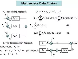
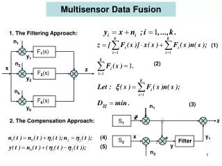
Multisensor Data Fusion
n 1. F 1 (s). y 1. n 2. x. z. F 2 (s). y 2. n k. F k (s). n 1. y k. x. x. z. S 1. x. y 1. +. S 2. Filter. -. y. n 2. 1. The Filtering Approach:. (1). Multisensor Data Fusion. (2). (3). 2. The Compensation Approach:. (4). +. (5). a. Goals of Optimization.

Multisensor Data Fusion
E N D
Presentation Transcript
n1 F1(s) y1 n2 x z F2(s) y2 nk Fk(s) n1 yk x x z S1 x y1 + S2 Filter - y n2 1. The Filtering Approach: (1) Multisensor Data Fusion (2) (3) 2. The Compensation Approach: (4) + (5)
a Goals of Optimization 1. Unbiasedness: (5) (6) 2. Minimal variance:
Kalman Filter Built-in to the Commercial Navigation Measurement System
Kalman Filter GPS+SINS Integration Sensors SINS GPS State Space Equations of SINS Errors: (7) (8)
Measurement: (9) where: Mathematical Formulation of the Kalman Filtering Problem (10) (11) Let: Filtration error: (12) Prediction:
Main Requirements: (13) 1. Zero-bias (see (5)): (14) 2. Minimal Variance: Prediction error (derived from (10) and (12)) : Covariance matrix of prediction error : (15) (16) Estimation of the prediction based on the measurement results (measurement update): (17) (18)
From (13) it follows: (19) (20) From (13) and (20) it follows: (21) Substituting (21) in (17), we obtain: (22) Determination of the Kalman Gain K from requirement (14) (23) (25) Substituting (11) in (25), we obtain: (26)
(27) Condition of optimality: (28) Differentiation of the traces of matrices: (29) (30) (31) Taking in account (30) and (31), expression (27) can be simplified: (32) Basic expression for Kalman Filtering are: (12), (16), (22), (31), (32).
z-1 z-1 Time-dependant Kalman Filter Algorithm 1 P(0),X(0),n, Hn,Qn,Rn. Initial data: (16) (12) Measurements (31) y[n] (32) (22) 7
(33) Discrete Stationary Kalman Filter (34) Command in MATLAB for discrete models (3): [kest, K, P, M, Z]=kalman(‘sys’,Q,R) (35)
Block Diagram of Discrete Kalman Filter y [ n ] e e K H ( 1 / z )* I text [ [ /n-1] ] n n Y Y X [ n / n - 1 ] M H
Example: fusion of the dead reckon and radio-navigation systems v w1 FK RNS w2 DRS yn w (1) (2) (3)
n1 F1(s) y1 n2 x z F2(s) y2 nk Fk(s) yk Multisensor Data Fusion The Filtering Approach: (1) (2) (3)
n y e W(s) F(s) x I(s)=1 Optimal Filtration in Scalar Case. (4) (5) Wiener-Hopf Equation: (6) (6a) (7)
Wiener Factorization: (8) Wiener Separation: (9) Optimal Filter: (10) Example: (11) (12) (13)
n W(s) F(s) x y n1 z F1(s) W1(s) y1 ε Optimal Fusion of 2 sensors. (1) i (2) (3) (4) (5) (6)
Wiener-Hopf equation: (7) (8) (9) Example: fusion of Doppler and barometric speed sensors: Barometric: (10) (11) Doppler: (12) where:
General Block Diagram of the Information Processing in the ACS. BITE Sources of Infor- mation (sensors) Sources of Infor- mation (sensors) PP SP&AS ToI Receiver
CDN Computer Network Architecture of Boeing-787 CCR Remote Data Concentrators
Example: 3-digit word Dec. Bin. Grey 0 0 0 0 0 0 0 y 1 0 0 1 0 0 1 2 0 1 0 0 1 1 x 0 1 3 0 1 1 0 1 0 0 0 1 4 1 0 0 1 1 0 1 1 0 5 1 0 1 1 1 1 6 1 1 0 1 0 1 7 1 1 1 1 0 0 Max Hd= 1. Hd=3 1. Coding of Signals. Hamming’s distance: Grey Code. Transmission of Information Encoding: Truth Table: Decoding:
Angle-Code Converter BINARY ENCODER GRAY ENCODER
Com. Ch. LPF CSG ym ym 2. Modulation of Signals