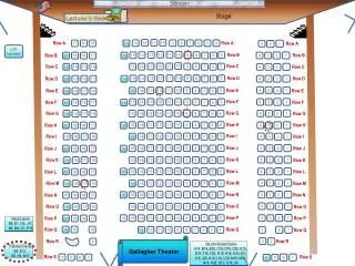
Stage
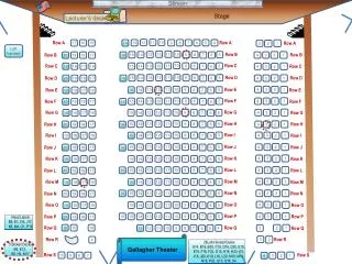
Stage. Screen. Lecturer’s desk. 11. 10. 9. 8. 7. 6. 5. 2. 14. 13. 12. 4. 3. 1. Row A. 14. 13. 12. 11. 10. 9. 6. 8. 7. 5. 4. 3. 2. 1. Row B. 28. 27. 26. 23. 25. 24. 22. Row C. 7. 6. 5. Row C. 2. 4. 3. 1. 21. 20. 19. 18. 17. 16. 13. Row C. 15.

Stage
E N D
Presentation Transcript
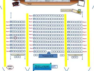
Stage Screen Lecturer’s desk 11 10 9 8 7 6 5 2 14 13 12 4 3 1 Row A 14 13 12 11 10 9 6 8 7 5 4 3 2 1 Row B 28 27 26 23 25 24 22 Row C 7 6 5 Row C 2 4 3 1 21 20 19 18 17 16 13 Row C 15 14 12 11 10 9 8 22 27 28 26 25 24 23 Row D 1 Row D 6 21 20 19 18 17 16 13 7 5 4 3 2 15 14 12 11 10 9 8 Row D Row E 28 27 26 22 Row E 23 25 24 7 6 5 1 2 4 3 Row E 21 20 19 18 17 16 13 15 14 12 11 10 9 8 Row F 28 27 26 23 25 24 22 Row F 1 6 21 20 19 18 17 16 13 7 5 4 3 2 15 14 12 11 10 9 8 Row F Row G 22 27 28 26 25 24 23 7 6 5 1 Row G 2 4 3 Row G 21 20 19 18 17 16 13 15 14 12 11 10 9 8 Row H 28 27 26 22 23 25 24 Row H 6 21 20 19 18 17 16 13 7 5 4 3 2 1 15 14 12 11 10 9 8 Row H Row J 28 27 26 23 25 24 22 7 6 5 Row J 2 4 3 1 Row J 21 20 19 18 17 16 13 15 14 12 11 10 9 8 22 27 28 26 25 24 23 6 21 20 19 18 17 16 13 7 5 4 3 2 1 15 14 12 11 10 9 8 Row K Row K Row K 28 27 26 22 23 Row L 25 24 21 20 19 18 17 16 13 6 15 14 12 11 10 9 8 Row L 7 5 4 3 2 1 Row L 28 27 26 22 23 Row M 25 24 21 20 19 18 17 16 13 6 12 11 10 9 8 Row M 7 5 4 3 2 1 Row M table • Projection Booth 14 13 2 1 table 3 2 1 3 2 1 Modern Languages ML350 Renumbered R/L handed broken desk
MGMT 276: Statistical Inference in ManagementRoom 350 Modern LanguagesSpring, 2012 Welcome
Homework 13: Using Excel to complete ANOVAs Due Tuesday, April 17th Homework 14: ANOVA Project Using Excel to complete your own ANOVA project Due Thursday, April 19th Please click in My last name starts with a letter somewhere between A. A – D B. E – L C. M – R D. S – Z Please double check – All cell phones other electronic devices are turned off and stowed away
Use this as your study guide Next couple of lectures 4/17/12 Hypothesis testing with analysis of variance (ANOVA) Interpreting excel output of hypothesis tests Constructing brief, complete summary statements Logic of hypothesis testing with Correlations Interpreting the Correlations and scatterplots Simple and Multiple Regression Using correlation for predictions Regression uses the predictor variable (independent) to make predictions about the predicted variable (dependent)Coefficient of correlation is name for “r”Coefficient of determination is name for “r2”(remember it is always positive – no direction info)Standard error of the estimate is our measure of the variability of the dots around the regression line(average deviation of each data point from the regression line – like standard deviation) Coefficient of regression will “b” for each variable (like slope)
Readings for next exam (Exam 4 is on 4/26/12) Lind Chapter 12: Analysis of Variance Chapter 13: Linear Regression and Correlation Chapter 14: Multiple Regression Chapter 15: Chi-Square Plous Chapter 17: Social Influences Chapter 18: Group Judgments and Decisions
Exam 4 – Optional Final Time • Two options for completing Exam 4 • Thursday (4/26/12) • Tuesday (5/1/12) • Must sign up to take the later Exam 4 by Tuesday (4/24) • Only need to take one exam – these are two optional times
Type of major in school 4 (accounting, finance, hr, marketing) Grade Point Average Homework 0.05 2.83 3.02 3.24 3.37
0.3937 0.1119 If observed F is bigger than critical F:Reject null & Significant! If observed F is bigger than critical F:Reject null & Significant! 0.3937 / 0.1119 = 3.517 Homework 3.517 3.009 If p value is less than 0.05:Reject null & Significant! 3 24 0.03 4-1=3 # groups - 1 # scores - number of groups 28 - 4=24 # scores - 1 28 - 1=27
Yes Homework = 3.517; p < 0.05 F (3, 24) The GPA for four majors was compared. The average GPA was 2.83 for accounting, 3.02 for finance, 3.24 for HR, and 3.37 for marketing. An ANOVA was conducted and there is a significant difference in GPA for these four groups (F(3,24) = 3.52; p < 0.05).
Average for each group(We REALLY care about this one) Number of observations in each group Just add up all scores (we don’t really care about this one)
Number of groups minus one(k – 1) 4-1=3 “SS” = “Sum of Squares”- will be given for exams Number of people minus number of groups (n – k) 28-4=24
SS between df between SS within df within MS between MS within
Type of executive 3 (banking, retail, insurance) Hours spent at computer 0.05 10.8 8 8.4
11.46 2 If observed F is bigger than critical F:Reject null & Significant! If observed F is bigger than critical F:Reject null & Significant! 11.46 / 2 = 5.733 5.733 3.88 If p value is less than 0.05:Reject null & Significant! 2 12 0.0179
Yes p < 0.05 F (2, 12) = 5.73; The number of hours spent at the computer was compared for three types of executives. The average hours spent was 10.8 for banking executives, 8 for retail executives, and 8.4 for insurance executives. An ANOVA was conducted and we found a significant difference in the average number of hours spent at the computer for these three groups , (F(2,12) = 5.73; p < 0.05).
Average for each group(We REALLY care about this one) Number of observations in each group Just add up all scores (we don’t really care about this one)
Number of groups minus one(k – 1) 3-1=2 “SS” = “Sum of Squares”- will be given for exams Number of people minus number of groups (n – k) 15-3=12
SS between df between SS within df within MS between MS within
Let’s try one In a one-way ANOVA we have three types of variability. Which picture best depicts the random error variability (also known as the within variability)? a. Figure 1 b. Figure 2 c. Figure 3 d. All of the above 1. 2. 3.
Variability between groups F = Let’s try one Variability within groups Which figure would depict the largest F ratio a. Figure 1 b. Figure 2 c. Figure 3 d. All of the above 1. 2. 3.
Let’s try one Winnie found an observed F ratio of .9, what should she conclude? a. Reject the null hypothesis b. Do not reject the null hypothesis c. Not enough info is given 1. 2. 3.
How many observations within each group? Let’s try one An ANOVA was conducted comparing different types of solar cells and there appears to be a significant difference in output of each (watts) F(4, 25) = 3.12; p < 0.05. In this study there were __ types of solar cells and __ total observations in the whole study? a. 4; 25 b. 5; 30 c. 4; 30 d. 5; 25 F(4, 25) = 3.12; p < 0.05 # groups - 1 # scores - # of groups # scores - 1
Let’s try one An ANOVA was conducted comparing different types of solar cells and there appears to be significant difference in output of each (watts) F(4, 25) = 3.12; p < 0.05. In this study ___ a. we rejected the null hypothesis b. we did not reject the null hypothesis F(4, 25) = 3.12; p < 0.05 Observed F bigger than Critical F p < .05
Let’s try one An ANOVA was conducted comparing different types of solar cells. The analysis was completed using an alpha of 0.05. But Julia now wants to know if she can reject the null with an alpha of at 0.01. In this study ___ a. we rejected the null hypothesis b. we did not reject the null hypothesis F(4, 25) = 3.12; p < 0.05 Comparison of the Observed F and Critical F Is no longer are helpful because the critical F is no longer correct. We must use the p value p < .05 p > .01
Let’s try one An ANOVA was conducted comparing home prices in four neighborhoods (Southpark, Northpark, Westpark, Eastpark) . For each neighborhood we measured the price of four homes. Please complete this ANOVA table. Degrees of freedom between is _____; degrees of freedom within is ____ a. 16; 4 b. 4; 16 c. 12; 3 d. 3; 12 .
Let’s try one An ANOVA was conducted comparing home prices in four neighborhoods (Southpark, Northpark, Westpark, Eastpark) . For each neighborhood we measured the price of four homes. Please complete this ANOVA table. Mean Square between is _____; Mean Square within is ____ a. 300, 300 b. 100, 100 c. 100, 25 d. 25, 100 .
Let’s try one An ANOVA was conducted comparing home prices in four neighborhoods (Southpark, Northpark, Westpark, Eastpark) . For each neighborhood we measured the price of four homes. Please complete this ANOVA table. The F ratio is: a. .25 b. 1 c. 4 d. 25 .
Let’s try one An ANOVA was conducted comparing home prices in four neighborhoods (Southpark, Northpark, Westpark, Eastpark) . For each neighborhood we measured the price of four homes. Please complete this ANOVA table. We should: a. reject the null hypothesis b. not reject the null hypothesis Observed F bigger than Critical F p < .05
Let’s try one An ANOVA was conducted comparing home prices in four neighborhoods (Southpark, Northpark, Westpark, Eastpark) . For each neighborhood we measured the price of four homes. The most expensive neighborhood was the ____ neighborhood a. Southpark b. Northpark c. Westpark d. Eastpark
An ANOVA was conducted comparing home prices in four neighborhoods (Southpark, Northpark, Westpark, Eastpark) . For each neighborhood we measured the price of four homes. Please complete this ANOVA table. The best summary statement is: a. F(3, 12) = 4.0; n.s. b. F(3, 12) = 4.0; p < 0.05 c. F(3, 12) = 3.49; n.s. d. F(3, 12) = 3.49; p < 0.05
A t-test was conducted to see whether “Bankers” or “Retailers” spend more time in front of their computer. Which best summarizes the results from this excel output: a. Bankers spent significantly more time in front of their computer screens than Retailers, t(3.5) = 8; p < 0.05 b. Bankers spent significantly more time in front of their computer screens than Retailers, t(8) = 3.5; p < 0.05 c. Retailers spent significantly more time in front of their computer screens than Bankers, t(3.5) = 8; p < 0.05 d. Retailers spent significantly more time in front of their computer screens than Bankers, t(8) = 3.5; p < 0.05 e. There was no difference between the groups
Let’s try one A t-test was conducted to see whether “Bankers” or “Retailers” spend more time in front of their computer. Which critical t would be the best to use a. 3.5 b. 1.859 c. 2.306 d. .004 e. .008
Let’s try one An ANOVA was conducted and there appears to be a significant difference in the number of cookies sold as a result of the different levels of incentive F(2, 27) = ___; p < 0.05. Please fill in the blank a. 3.3541 b. .00635 c. 6.1363 d. 27.00
An ANOVA was conducted and we found the following results: F(3,12) = 3.73 ____. Which is the best summary a. The critical F is 3.89; we should reject the null b. The critical F is 3.89; we should not reject the null c. The critical F is 3.49; we should reject the null d. The critical F is 3.49; we should not reject the null Let’s try one
Five steps to hypothesis testing Step 1: Identify the research problem (hypothesis) Describe the null and alternative hypotheses For correlation null is that r = 0 (no relationship) Step 2: Decision rule • Alpha level? (α= .05 or .01)? • Critical statistic (e.g. critical r) value from table? Step 3: Calculations MSBetween F = MSWithin Step 4: Make decision whether or not to reject null hypothesis If observed r is bigger then critical r then reject null Step 5: Conclusion - tie findings back in to research problem
Finding a statistically significant correlation • The result is “statistically significant” if: • the observed correlation is larger than the critical correlationwe want our r to be big if we want it to be significantly different from zero!! (either negative or positive but just far away from zero) • the p value is less than 0.05 (which is our alpha) • we want our “p” to be small!! • we reject the null hypothesis • then we have support for our alternative hypothesis
Correlation Correlation: Measure of how two variables co-occur and also can be used for prediction • Range between -1 and +1
Correlation • The closer to zero the weaker the relationship and the worse the prediction • Positive or negative
Positive correlation • Positive correlation: • as values on one variable go up, so do values for other variable • pairs of observations tend to occupy similar relative positions • higher scores on one variable tend to co-occur with higher scores on the second variable • lower scores on one variable tend to co-occur with lower scores on the second variable • scatterplot shows clusters of point • from lower left to upper right
Negative correlation • Negative correlation: • as values on one variable go up, values for other variable go down • pairs of observations tend to occupy dissimilar relative positions • higher scores on one variable tend to co-occur with lower scores on • the second variable • lower scores on one variable tend to • co-occur with higher scores on the • second variable • scatterplot shows clusters of point • from upper left to lower right
Zero correlation • as values on one variable go up, values for the other variable • go... anywhere • pairs of observations tend to occupy seemingly random • relative positions • scatterplot shows no apparent slope
http://www.ruf.rice.edu/~lane/stat_sim/reg_by_eye/index.html http://argyll.epsb.ca/jreed/math9/strand4/scatterPlot.htm Let’s estimate the correlation coefficient for each of the following r = +.98 r = .20
http://www.ruf.rice.edu/~lane/stat_sim/reg_by_eye/index.html http://argyll.epsb.ca/jreed/math9/strand4/scatterPlot.htm Let’s estimate the correlation coefficient for each of the following r = +. 83 r = -. 63