Download
1 / 12
120 likes | 281 Views
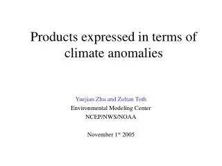
Products expressed in terms of climate anomalies. Yuejian Zhu and Zoltan Toth Environmental Modeling Center NCEP/NWS/NOAA November 1 st 2005. Input climate/forecast data -- current available. NCEP/NCAR reanalysis data 4 cycles (00UTC, 06UTC, 12UTC and 18UTC) per day

E N D
Products expressed in terms of climate anomalies Yuejian Zhu and Zoltan Toth Environmental Modeling Center NCEP/NWS/NOAA November 1st 2005
Input climate/forecast data -- current available • NCEP/NCAR reanalysis data • 4 cycles (00UTC, 06UTC, 12UTC and 18UTC) per day • 40 years (Jan. 1st 1959 – Dec. 31th 1998) • Need to consider the systematic difference between NCEP/NCAR reanalysis and current analysis (GDAS) • Resolution and format • 2.5*2.5 (lat/lon) grid, GRIB-1 format • 1.0*1.0 (lat/lon) grid, GRIB-1 format (forecast only) • Variables at levels (possible to add more) • Height: 1000hPa, 700hPa, 500hPa, 250hPa • Temperature: 2m, 850hPa, 500hPa, 250hPa • Wind: 10m, 850hPa, 500hPa, 250hPa • PRMSL,max/min temperature
Climatological mean (estimation) • To use Fourier expansion from 40 years data and compare following four considerations • Considering first Fourier mode: a1 and b1 • Fits to daily data to obtain annual cycle • Considering first two Fourier modes: a1,b1,a2 and b2 • Fits to daily data to obtain annual and semi-annual cycle • Considering first three Fourier modes: a1,b1,a2,b2,a3 and b3 • Fits to daily data to obtain annual, semi-annual and 4-month cycle • Considering first four Fourier modes: a1,b1,a2,b2,a3,b3,a4 and b4 • Fits to daily data to obtain annual, semi-annual, 4-month and seasonal cycle
Higher moments (estimation)- work on the anomalies from mean • Standard deviations: • Based on 4 different daily means (previous slide) • To get 40 years average daily standard deviation first • To calculate monthly mean of standard deviation from daily • To generate a slope from month to month • To project to daily standard deviation from month mean
Products (plan) • Based on 4 different considerations (choose one) • Assuming the normal distributions of the 40 years climate data • PDF will be presented by first two moments (mean and standard deviation) • Considering the systematic differences between NCEP/NCAR reanalysis and current GDAS • Using bias corrected forecasts • To calculate climate anomaly: • For 1x1 degree grid point globally. • For all 19 variables (height, temperature, wind and etc.) • For each ensemble member. • Output in percentile (0-100%, 50%=normal).
Discussion • How many modes we need to consider? • In general, more modes will be better • First two modes are enough for the heights • Surface variables and winds are challenged • Are all variables normal distribution? • Depends on variables and geographical locations (?) • Most of them are normal distribution • Examples of 2-meter temperature and 10-meter u • Monthly distribution of 500hPa height has a little seasonal tilt • Examples of time series for daily mean and standard deviation for all 19 selected variables • Two physical locations (near Washington DC and Ottawa) • Are these plots enough to demonstrate? • http://wwwt.emc.ncep.noaa.gov/gmb/yzhu/html/CLIMATE_ANOMALY.html
Notes for presentation and posted maps • Next few slides are from early studies • Based on monthly average of climatology • Using L-moment and several fitting methods • Probabilistic extreme forecasts are for future NDGD purpose • Examples of future application for NAEFS • Visit http://wwwt.emc.ncep.noaa.gov/gmb/yzhu/html/CLIMATE_ANOMALY.html • For four different modes consideration (need choose one only) • January 15th and July 15th are posted to contrast of seasonal difference • 0000UTC and 1200UTC are posted to contrast of daily cycle • November 1st 0000UTC 2005 raw forecasts are used as example • Only one ensemble member is demonstrated • Differences (reanalysis and GDAS) are not considered (not available yet) • Bias corrected forecasts will be used when final application • Anomaly forecast maps are shown normal (0%), above normal (+%) and below normal (-%) respectively • Maximum and minimum temperatures • Not quite right! 6 hours climate .vs 12 hours forecast (only available right now) • 6 hours tmax and tmin will be generated soon for ensemble system.
Climatological mean and higher moments-Early study • To consider monthly mean (tested) • Monthly mean (large data samples – 1240) • Interpolate to daily (shifted from season) • To consider daily mean (tested) • 5-day running mean for daily climatology • Data samples – 200 • 5-day center weighted mean for monthly climatology • Data samples – 200 • (d-2)*0.12+(d-1)*0.22+d*0.32+(d+1)*0.22+(d+2)*0.12 • Fitting distributions (three parameters) • Gamma, Pearson type-III, GE3 (generalized extreme-value)
GEV Monthly mean 5-day weighted mean
GEV Monthly mean 5-day weighted mean
GEV PE3 PE3 Monthly mean 5-day weighted mean
ENSEMBLE 10-, 50- (MEDIAN) & 90-PERCENTILE FORECAST VALUES (BLACK CONTOURS) AND CORRESPONDING CLIMATE PERCENTILES (SHADES OF COLOR) Example of probabilistic forecast in terms of climatology