Download
1 / 51
560 likes | 839 Views
IE 337: Materials & Manufacturing Processes. Lecture 4: Mechanics of Metal Cutting. Chapter 21. Last Time. Assignment #1 – Due Tuesday 1/19 How we can modify mechanical properties in metals? Alloying Annealing controlling grain size (recrystallization and grain growth)

E N D
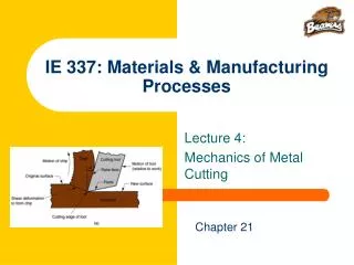
IE 337: Materials & Manufacturing Processes Lecture 4: Mechanics of Metal Cutting Chapter 21
Last Time • Assignment #1 – Due Tuesday 1/19 • How we can modify mechanical properties in metals? • Alloying • Annealing • controlling grain size (recrystallization and grain growth) • phase dispersion (coarse vs fine pearlite) • Allotropic transformation – austenite to martensite • Precipitation hardening • (Grain size refinement) • Different types of metal alloys and how they are used?
Recrystallization and Grain Growth Scanning electron micrograph taken using backscattered electrons, of a partly recrystallized Al-Zr alloy. The large defect-free recrystallized grains can be seen consuming the deformed cellular microstructure. --------50µm-------
Figure 6.4 Phase diagram for iron‑carbon system, up to about 6% carbon. Allotropic Transformation and Tempering Austenizing Quenching Tempered Martensite 5
Precipitation Hardening - Al 6022 (Mg-Si) Figure 27.5 Precipitation hardening: (a) phase diagram of an alloy system consisting of metals A and B that can be precipitation hardened; and (b) heat treatment: (1) solution treatment, (2) quenching, and (3) precipitation treatment. 6
This Time • How do we shape materials? • Secondary operations Material Removal • The fundamentals of metal cutting (Chapter 21) • Chip formation • Orthogonal machining • The Merchant Equation • Power and Energy in Machining • Cutting Temperature
Material Removal Processes A family of shaping operations, the common feature of which is removal of material from a starting workpart to create a desired shape • Categories: • Machining – material removal by a sharp cutting tool, e.g., turning, milling, drilling • Abrasive processes – material removal by hard, abrasive particles, e.g., grinding • Nontraditional processes - various energy forms other than sharp cutting tool to remove material
Variety of work materials can be machined Most frequently applied to metals Variety of part shapes and special geometry features possible, such as: Screw threads Accurate round holes Very straight edges and surfaces Good dimensional accuracy and surface finish Wasteful of material Chips generated in machining are wasted material, at least in the unit operation Time consuming A machining operation generally takes more time to shape a given part than alternative shaping processes, such as casting, powder metallurgy, or forming Machining
Classification of Machined Parts Machined parts are classified as: (a) rotational, or (b) nonrotational, shown here by block and flat parts
Turning • Single point cutting tool removes material from a rotating workpiece to form a cylindrical shape
Milling • Rotating multiple-cutting-edge tool is moved slowly relative to work to generate plane or straight surface • Two forms: peripheral milling and face milling
Drilling • Used to create a round hole, usually by means of a rotating tool (drill bit) that has two cutting edges
Machine Tools A power‑driven machine that performs a machining operation, including grinding • Functions in machining: • Holds workpart • Positions tool relative to work • Provides power at speed, feed, and depth that have been set • The term is also applied to machines that perform metal forming operations 14
Cutting Tools Typical hot hardness relationships for selected tool materials.
Cutting Fluids • Functions • Cooling • Lubrication • Flush debris • Types • Coolants • Water used as base in coolant‑type cutting fluids • Most effective at high cutting speeds where heat generation and high temperatures are problems • Most effective on tool materials that are most susceptible to temperature failures (e.g., HSS) • Lubricants • Usually oil‑based fluids • Most effective at lower cutting speeds • Also reduces temperature in the operation
Cutting Conditions in Machining • Three dimensions of a machining process: • Cutting speed v – primary motion • Feed f – secondary motion • Depth of cut d – penetration of tool below original work surface • For turning operations, material removal rate can be computed as RMR = v f d where v = cutting speed; f = feed; d = depth of cut 17
Cutting Conditions for Turning Figure 21.5 Speed, feed, and depth of cut in turning. 18
Roughing vs. Finishing In production, several roughing cuts are usually taken on the part, followed by one or two finishing cuts • Roughing - removes large amounts of material from starting workpart • Creates shape close to desired geometry, but leaves some material for finish cutting • High feeds and depths, low speeds • Finishing - completes part geometry • Final dimensions, tolerances, and finish • Low feeds and depths, high cutting speeds 19
Orthogonal Cutting Model Simplified 2-D model of machining that describes the mechanics of machining fairly accurately Figure 21.6 Orthogonal cutting: (a) as a three‑dimensional process. 20
Chip Formation Figure 21.8 More realistic view of chip formation, showing shear zone rather than shear plane. Also shown is the secondary shear zone resulting from tool‑chip friction. 21
Chip Types • Discontinuous chip • Continuous chip • Continuous chip with Built-up Edge (BUE) • Serrated chip
Discontinuous Chip • Brittle work materials (e.g., cast irons) • Low cutting speed • Large feed • Large depth of cut • High tool‑chip friction Four types of chip formation in metal cutting: (a) discontinuous
Continuous Chip • Ductile work materials (e.g., low carbon steel) • High cutting speeds • Small feeds and depths • Sharp cutting edge on the tool • Low tool‑chip friction Four types of chip formation in metal cutting: (b) continuous
Continuous with BUE • Ductile materials • Low‑to‑medium cutting speeds • Tool-chip friction causes portions of chip to adhere to rake face • BUE formation is cyclical; it forms, then breaks off Four types of chip formation in metal cutting: (c) continuous with built‑up edge
Serrated Chip • Semi-continuous - saw-tooth appearance (e.g. Ti alloys) • Cyclical chip formation of alternating high shear strain then low shear strain • Most closely associated with difficult-to-machine metals at high cutting speeds Four types of chip formation in metal cutting: (d) serrated
Determining Shear Plane Angle • Based on the geometric parameters of the orthogonal model, the shear plane angle can be determined as: where r = chip ratio and = rake angle 27
Chip Thickness Ratio where r = chip thickness ratio; to = thickness of the chip prior to chip formation; and tc = chip thickness after separation • Chip thickness after cut always greater than before, so chip ratio always less than 1.0 28
Shear Strain in Chip Formation Figure 21.7 Shear strain during chip formation: (a) chip formation depicted as a series of parallel plates sliding relative to each other, (b) one of the plates isolated to show shear strain, and (c) shear strain triangle used to derive strain equation. 29
Shear Strain Shear strain in machining can be computed from the following equation, based on the preceding parallel plate model: • = tan( - ) + cot where = shear strain, = shear plane angle, and = rake angle of cutting tool 30
Chip Formation Figure 21.8 More realistic view of chip formation, showing shear zone rather than shear plane. Also shown is the secondary shear zone resulting from tool‑chip friction. 31
Forces Acting on Chip • Friction force F and Normal force to friction N • Shear force Fs and Normal force to shear Fn Figure 21.10 Forces in metal cutting: (a) forces acting on the chip in orthogonal cutting 32
Resultant Forces • Vector addition of F and N = resultant R • Vector addition of Fs and Fn = resultant R' • Forces acting on the chip must be in balance: • R' must be equal in magnitude to R • R’ must be opposite in direction to R • R’ must be collinear with R 33
Coefficient of Friction Coefficient of friction between tool and chip: Friction angle related to coefficient of friction as follows: 34
Shear Stress Shear stress acting along the shear plane: where As = area of the shear plane Shear stress = shear strength of work material during cutting 35
Cutting Force and Thrust Force • F, N, Fs, and Fn cannot be directly measured • Forces acting on the tool that can be measured: • Cutting force Fc and Thrust force Ft Figure 21.10 Forces in metal cutting: (b) forces acting on the tool that can be measured 36
Forces in Metal Cutting • Equations can be derived to relate the forces that cannot be measured to the forces that can be measured: F = Fc sin + Ft cos N = Fc cos ‑ Ft sin Fs = Fc cos ‑ Ft sin Fn = Fc sin + Ft cos • Based on these calculated force, shear stress and coefficient of friction can be determined 37
The Merchant Equation • Of all the possible angles at which shear deformation can occur, the work material will select a shear plane angle that minimizes energy, given by • Derived by Eugene Merchant • Based on orthogonal cutting, but validity extends to 3-D machining 38
What the Merchant Equation Tells Us • To increase shear plane angle • Increase the rake angle • Reduce the friction angle (or coefficient of friction) 39
Effect of Higher Shear Plane Angle • Higher shear plane angle means smaller shear plane which means lower shear force, cutting forces, power, and temperature Figure 21.12 Effect of shear plane angle : (a) higher with a resulting lower shear plane area; (b) smaller with a corresponding larger shear plane area. Note that the rake angle is larger in (a), which tends to increase shear angle according to the Merchant equation 40
Power and Energy Relationships • A machining operation requires power • The power to perform machining can be computed from: Pc = Fc v where Pc = cutting power; Fc = cutting force; and v = cutting speed 41
Power and Energy Relationships • In U.S. customary units, power is traditional expressed as horsepower (dividing ft‑lb/min by 33,000) where HPc = cutting horsepower, hp 42
Power and Energy Relationships • Gross power to operate the machine tool Pg or HPg is given by or • where E = mechanical efficiency of machine tool • Typical E for machine tools 90% 43
Unit Power in Machining • Useful to convert power into power per unit volume rate of metal cut • Called unit power, Pu or unit horsepower, HPu or where RMR = material removal rate 44
Specific Energy in Machining Unit power is also known as the specificenergyU Units for specific energy are typically N‑m/mm3 or J/mm3 (in‑lb/in3) 45
Cutting Temperature • Approximately 98% of the energy in machining is converted into heat • This can cause temperatures to be very high at the tool‑chip • The remaining energy (about 2%) is retained as elastic energy in the chip 46
Cutting Temperatures are Important High cutting temperatures • Reduce tool life • Produce hot chips that pose safety hazards to the machine operator • Can cause inaccuracies in part dimensions due to thermal expansion of work material 47
Cutting Temperature • Analytical method derived by Nathan Cook from dimensional analysis using experimental data for various work materials where T = temperature rise at tool‑chip interface; U = specific energy; v = cutting speed; to = chip thickness before cut; C = volumetric specific heat of work material; K = thermal diffusivity of work material 48
Cutting Temperature • Experimental methods can be used to measure temperatures in machining • Most frequently used technique is the tool‑chip thermocouple • Using this method, Ken Trigger determined the speed‑temperature relationship to be of the form: T = K vm where T = measured tool‑chip interface temperature, and v = cutting speed 49
You should have learned: • The fundamentals of metal cutting (Chapter 21) • Chip formation • Orthogonal machining • The Merchant Equation • Power and Energy in Machining • Cutting Temperature