Transforming Kinematics Learning: Experiential Insights from MBL Activities
Explore how MBL activities transform kinematics learning based on a study with Year 11 physics students using a predict-Observe-Explain format. Discover students' innovative data manipulation techniques and the deep engagement enabled by the use of graphic displays.

Transforming Kinematics Learning: Experiential Insights from MBL Activities
E N D
Presentation Transcript
Physics E-lab:Distance and Time Session 3 April 29th EDCP 447 N. Jahng
Literature Review • Russell, Lucas, & McRobbie (2003) • Problem: Teachers’ failure to utilise MBL activities may be due to not recognising their capacity to transform the nature of laboratory activities to be more consistent with contemporary constructivist theories of learning. • Sample: Year 11 physics students (n=29) • Context: Kinematics activities using a predict-Observe-Explain format • Data: video and audio recordings of students and teacher, students’ display graphs and written notes, interviews, and the teacher’s journal • Findings: • Many instances where students’ initial understanding of kinematics were mediated in multiple ways • Students invented numerous techniques for manipulating data in the service of their emerging understanding.
ASSERTION 1. Students viewed the display, almost exclusively, as representing the experimental phenomena or task problem. (p. 226-7)
ASSERTION 2. During student-display interactions, …, the dyads completed the majority of tasks at a deep level of mental engagement. (p. 227-8)
Assertions 3-8 3. The enduring nature of the display was supportive of a deep approach to learning. 4. Students critically evaluated the appearance of the graphic display. 5. Learning conditions in the MBL were conducive to fostering conceptual change, the conditions being: graphic evidence to engender dissatisfaction with prior conceptions; opportunities to construct new conceptions that can be seen to be plausible, intelligible and fruitful; and an atmosphere that was motivationally and socially conducive to constructing new understandings. 6. Within and between groups, students used the screen as a shared resource to engage in a broad range of activities directed at creating and interpreting graphs. 7. The kinematics graphic display supported students’ working memory 8. The teacher’s probing questions stimulated deeply processed responses linked to graph features and the experimental phenomena.
Motion & Force • Three Laws of Motion • Newton's Laws of Motion illustrated with 3D animations and motion graphics • PASCO e-lab Force and Motion
Position & Time: Lab (1) • PURPOSE • to introduce the relationships between the motion of an object (position) and time • PROCEDURE • You will be the object in motion. The Motion Sensor will measure your position as you move in a straight line at different speeds. The Science Workshop program will plot your motion on a graph of position and time. The challenge in this activity is to move in such a way that a plot of your motion on the same graph will “match” the line that is already there.
PART I: Computer Setup • Connect the Science Workshop interface to the computer, • Connect the motion sensor’s stereo phone yellow-taped plug to Digital Channel 1 and the other plug to Digital Channel 2. • Open the Science Workshop • Select “Create Experiment” from the Startup screen • Select “New Activity” from the File menu • Click the “Setup” button • Click on “Choose interface” tab>> Select Science Workshop 500 interface • Add sensor >> select the motion sensor • Check measurement types • Double click type of measurement on the displays pane
PART III: Data Analysis • Use the Statistics tools in the Graph to determine the slope of the best fit line for the middle section of your best position vs. time plot. Click the “Statistics” button and then click the “Autoscale” button to resize the graph to fit the data. • Use the mouse to click-and-draw a rectangle around the middle section of your plot. Use the “Statistics” menu button in the Statistics area of the Graph. Select “Linear Fit” from the Curve Fit menu to display the slope of the selected region of your position vs time plot. • The “a2” term of the equation in the Stats area is the slope of the selected region of motion. • The slope of this part of the position vs. time plot is the velocity during the selected region of motion. • Determine how well your plot of motion fits the plot that was already in the Graph. • Examine the “total abs. difference” (total absolute difference) and the chi^2 (goodness of fit) terms from the Statistics area.
QUESTIONS • In the Graph, what is the slope of the line of best fit for the middle section of your plot? • What is the description of your motion? (Example: “Constant speed for 2 seconds followed by no motion for 3 seconds, etc.”)
Position & Time: Lab (2) • Make sure the switch at the top of the Motion Sensor is set to “Far” or “Narrow.”
Data Collection Procedure • Motion Matching • Observe the position v. time graph. Adjust the incline of the ramp, the location of the Motion Sensor, and the starting position of the car to match the given data on the position v. time graph. • Press the Start button and put the car into motion. • Press the Stop button when appropriate. • Repeat steps 1-3 until the graphs match.
Analysis (a) • Making a Velocity-Time graph from the Position-Time graph: • Using the cursor, highlight a section of the data that was collected from the beginning of the data run. • Press the Scale-to-Fit button . • Select the Smart Tool . • Drag the Smart Cursor to a data point. Record the time value. • Move the Smart Tool away from the data point. • Select the Slope Tool . • Move the slope cursor over the same data point. Record this value. • With no data points highlighted, select the Scale-to-Fit button • Repeat steps 1-8 at least 10 more times and enter the values into the Velocity v. Time graph. Make sure the data points are evenly spaced.
Analysis (b) • Making a Velocity-Time graph from an Acceleration-Time graph: • Select the Smart Tool . • Drag the Smart Cursor to a data point. Record the time value. • Select the Statistics Tool. • Using the cursor, drag a rectangle from the first data point to the Smart Cursor so that the entire area in between is shaded. Note: the "Area" function of the Statistics Tool is already activated. • Enter the value in the Statistics window (not shown above) into the Velocity v. Time graph • Repeat steps 1-5 at least 10 more times and enter the values into the Velocity v. Time graph. Make sure the data points are evenly spaced.
PASCO physic experiments • 1-D Motion: Position vs Time 1-D Frame of Reference Constant Velocity Constant Acceleration Freefall • Newton's Laws: Newton's First Law Newton's Second Law Newton's Third Law Frictional Force • 2-D Motion: Projectile Motion Dynamics Systems