
Kriging philosophy
E N D
Presentation Transcript
Kriging philosophy • We assume that the data is sampled from an unknown function that obeys simple correlation rules. • The value of the function at a point is correlated to the values at neighboring points based on their separation in different directions. • The correlation is strong to nearby points and weak with far away points, but strength does not change based on location. • This is often grossly wrong because a function may be fast undulating in one corner of the design space and vary slowly in another corner. • Still, Kriging is a good surrogate, and it may be the most popular surrogate in academia. • Normally Kriging is used with the assumption that there is no noise so that it interpolates exactly the function values. • It works out to be a local surrogate, and it uses functions that are very similar to the radial basis functions.
Reminder: Covariance and Correlation • Covariance of two random variables X and Y • The covariance of a random variable with itself is the square of the standard deviation • Covariance matrix for a vector contains the covariances of the components • Correlation • The correlation matrix has 1 on the diagonal.
Correlation between function values at nearby points x=10*rand(1,10) 8.147 9.058 1.267 9.134 6.324 0.975 2.785 5.469 9.575 9.649 xnear=x+0.1; xfar=x+1; ynear=sin(xnear) 0.9237 0.2637 0.9799 0.1899 0.1399 0.8798 0.2538 -0.6551 -0.2477 -0.3185 y=sin(x) 0.9573 0.3587 0.9551 0.2869 0.0404 0.8279 0.3491 -0.7273 -0.1497 -0.2222 yfar=sin(xfar) 0.2740 -0.5917 0.7654 -0.6511 0.8626 0.9193 -0.5999 0.1846 -0.9129 -0.9405 rfar=corrcoef(y,yfar) 0.4229 r=corrcoef(y,ynear) 0.9894
Gaussian correlation function • Correlation between point x and point s y10=sin(10*x); y10near=sin(10*xnear) r10=corrcoef(y10,y10near) 0.4264 • For the function we would like to estimate
Linear trend model Systematic departure Sampling data points y Linear Trend Model Systematic Departure Kriging x Universal Kriging • Named after a South African mining engineer D. G. Krige • Assumption: Systematic departures Z(x) are correlated • Gaussian correlation function C(x,s,θ) is most popular
Simple Kriging • Kriging started without the trend, and it is not clear that one cannot get by without it. • Simple Kriging is uses a covariance structure with a constant standard deviation. • The most popular correlation structure is Gaussian • The standard deviation measures the uncertainty in function values. If we have dense data, that uncertainty will be small, and if the data is sparse the uncertaty will be large. • How do you decide whether the data is sparse or dense?
Prediction and shape functions • Simple Kriging prediction formula • R is the correlation matrix of the data points. • The equation is linear in r, which means that the basis functions are the exponentials • The equation is linear in y, which is in common with linear regression.
Prediction variance Square root of variance is still called standard error The uncertainty at any x is still normally distributed.
Finding the thetas • The thetas and sigma must be found by optimization. • Maximize the likelihood of the data. • For a given curve, we can calculate the probability that if the curve is exact, we would have sampled the data. • Minimize the cross-validation error. • Each set of theta acts like a different surrogate. • Both problems are ill-conditioned and expensive for large number of data points. • Watch for thetas reaching their higher bounds! • Prediction variance equation does not count for the uncertainty in the theta values.