Kriging
Kriging. Cost of surrogates. In linear regression, the process of fitting involves solving a set of linear equations once.

Kriging
E N D
Presentation Transcript
Cost of surrogates • In linear regression, the process of fitting involves solving a set of linear equations once. • With radial basis neural networks we have to optimize the selection of neurons, which will again entail multiple solutions of the linear system. We may find the best spread by minimizing cross-validation errors. • Kriging, our next surrogate is even more expensive, we have a spread constant in every direction and we have to perform optimization to calculate the best set of constants (hyperparameters). • With many hundreds of data points this can become significant computational burden.
Introduction to Kriging • Method invented in the 1950s by South African geologist Danie G. Krige (1919-2013) for predicting distribution of minerals. • Formalized by French engineer, Georges Matheron in 1960. • Statisticians refer to a more general Gaussian Process regression. • Became very popular for fitting surrogates to expensive computer simulations in the 21st century. • It is one of the best surrogates available. • It probably became popular late mostly because of the high computer cost of fitting it to data.
Kriging philosophy • We assume that the data is sampled from an unknown function that obeys simple correlation rules. • The value of the function at a point is correlated to the values at neighboring points based on their separation in different directions. • The correlation is strong to nearby points and weak with far away points, but strength does not change based on location. • Normally Kriging is used with the assumption that there is no noise so that it interpolates exactly the function values.
Reminder: Covariance and Correlation • Covariance of two random variables X and Y • The covariance of a random variable with itself is the square of the standard deviation. • Covariance matrix for a vector contains the covariances of the components. • Correlation • The correlation matrix has 1 on the diagonal.
Correlation between function values at nearby points for sine(x) • Generate 10 random numbers, translate them by a bit (0.1), and by more (1.0) x=10*rand(1,10) 8.147 9.058 1.267 9.134 6.324 0.975 2.785 5.469 9.575 9.649 xnear=x+0.1; xfar=x+1; • Calculate the sine function at the three sets. ynear=sin(xnear) 0.9237 0.2637 0.9799 0.1899 0.1399 0.8798 0.2538 -0.6551 -0.2477 -0.3185 y=sin(x) 0.9573 0.3587 0.9551 0.2869 0.0404 0.8279 0.3491 -0.7273 -0.1497 -0.2222 yfar=sin(xfar) 0.2740 -0.5917 0.7654 -0.6511 0.8626 0.9193 -0.5999 0.1846 -0.9129 -0.9405 • Compare corelations: r=corrcoef(y,ynear) 0.9894; rfar=corrcoef(y,yfar) 0.4229 • Decay to about 0.4 over one sixth of the wavelength. • Wavelength on sine function is 2~6
Gaussian correlation function • Correlation between point x and point s • We would like the correlation to decay to about 0.4 at one sixth of the wavelength . • Approximately • For the function we would like to estimate
Universal Kriging Trend model Systematic departure Sampling data points y Linear Trend Model Systematic Departure Kriging x • Trend function is most often a low order polynomial • We will cover Ordinary Kriging, where linear trend is just a constant to be estimated by data. • There is also Simple Kriging , where constant is assumed to be known (often as 0). • Assumption: Systematic departures Z(x) are correlated. • Kriging prediction comes with a normal distribution of the uncertainty in the prediction.
Notation • The function values are given at points , with the point having components (number of dimensions). • The function value at the ithpoint is =y(), and the vector of function values is denoted y. • Given decay rates , we form the covariance matrix of the data • The correlation matrix R above is formed from the covariance matrix, assuming a constant standard deviation which measures the uncertainty in function values. • For dense data, will be small, for sparse data will be large. • How do you decide whether the data is sparse or dense?
Prediction and shape functions • Ordinary Kriging prediction formula • The equation is linear in r, which means that the exponentials may be viewed as basis functions. • The equation is linear in the data y, in common with linear regression, but b is not calculated by minimizing RMS. • Note that far away from data (not good for substantial extrapolation).
Fitting the data • Fitting refers to finding the parameters • We fit by maximizing the likelihood that the data comes from a Gaussian process defined by . • Once they are found, the estimate of the mean and standard deviation is obtained as • Maximum likelihood is a tough optimization problem. • Some kriging codes minimize the cross validation error. • Stationary covariance assumption: smoothness of response is quite uniform in all regions of input space.
Prediction variance Square root of variance is called standard error. The uncertainty at any x is normally distributed. represents the mean of Kriging prediction.
Kriging fitting issues • The maximum likelihood or cross-validation optimization problem solved to obtain the kriging fit is often ill-conditioned leading to poor fit, or poor estimate of the prediction variance. • Poor estimate of the prediction variance can be checked by comparing it to the cross validation error. • Poor fits are often characterized by the kriging surrogate having large curvature near data points (see example on next slide). • It is recommended to visualize by plotting the kriging fit and its standard error.
Example of poor fits. True function Kriging Model Trend model : Covariance function :
selection Good fit and poor standard error SE: standard error
Kriging with nuggets • Nuggets – refers to the inclusion of noise at data points. • The more general Gaussian Process surrogates or Kriging with nuggets can handle data with noise (e.g. experimental results with noise).
Introduction to optimization with surrogates • Based on cycles. Each consists of sampling design points by simulations, fitting surrogates to simulations and then optimizing an objective. • Construct surrogate, optimize original objective, refine region and surrogate. • Typically small number of cycles with large number of simulations in each cycle. • Adaptive sampling • Construct surrogate, add points by taking into account not only surrogate prediction but also uncertainty in prediction. • Most popular, Jones’s EGO (Efficient Global Optimization). • Easiest with one added sample at a time.
Problems Kriging • Fit the quadratic function of Slide 13 with kriging using different options, like different covariance (different s) and trend functions and compare the accuracy of the fit. • For this problem compare the standard error with the actual error.