Forecasting for Operations
Forecasting for Operations. Dr. Everette S. Gardner, Jr. Forecasting for operations. Why we should forecast with models The importance of forecasting Exponential smoothing in a nutshell Case studies Customer service: U.S. Navy distribution system Inventory investment: Mfg. of snack foods


Forecasting for Operations
E N D
Presentation Transcript
Forecasting for Operations Dr. Everette S. Gardner, Jr.
Forecasting for operations Why we should forecast with models The importance of forecasting Exponential smoothing in a nutshell Case studies Customer service: U.S. Navy distribution system Inventory investment: Mfg. of snack foods Purchasing workload: Mfg. of water filtration systems Recommendations: How to improve forecast accuracy
Paper folding forecast A sheet of notebook paper is 1/100 of an inch thick. I fold the paper 40 times. How thick will it be after 40 folds?
The Importance of Forecasting Forecasts determine: Master schedules Economic order quantities Safety stocks JIT requirements to both internal and external suppliers
The Importance of Forecasting (cont.) Better forecast accuracy always cuts inventory investment. Example: Forecast accuracy is measured by the standard deviation of the forecast error Safety stocks are usually set at 3 times the standard deviation If the standard deviation is cut by $1, safety stocks are cut by $3
Exponential smoothing methods Forecasts are based on weighted moving averages of Level Trend Seasonality Averages give more weight to recent data
Origins of exponential smoothing Simple exponential smoothing – The thermostat model Error = Actual data – forecast New forecast = Old Forecast + (Weight x Error) Invented by Navy operations analyst Robert G. Brown in 1944 First application: Using sonar data to forecast the tracks of Japanese submarines
Exponential smoothing at work “A depth charge has a magnificent laxative effect on a submariner.” Lt. Sheldon H. Kinney, Commander, USS Bronstein (DE 189)
Forecast profiles from exponential smoothing Additive Multiplicative Nonseasonal Seasonality Seasonality Constant Level Linear Trend Exponential Trend Damped Trend
Automatic Forecasting with the damped trend In constant-level data, the forecasts emulate simple exponential smoothing:
Automatic Forecasting with the damped trend In data with consistent growth and little noise, the forecasts usually follow a linear trend:
Automatic Forecasting with the damped trend When the trend is erratic, the forecasts are damped:
Automatic Forecasting with the damped trend The damping effect increases with noise in the data:
Case 1: U.S. Navy distribution system Scope 50,000 line items stocked at 11 supply centers 240,000 demand series $425 million inventory investment Decision Rules Simple exponential smoothing Replenishment by economic order quantity Safety stocks set to minimize backorder delay time
Problems Customer pressure to reduce backorder delay No additional inventory budget available Characteristics of demand series 90% nonseasonal Frequent outliers and jump shifts in level Trends, usually erratic, in most series Solution Automatic forecasting with the damped trend U.S. Navy distribution system (cont.)
U.S. Navy distribution system (cont.) Research design 1 Random sample (5,000 items) selected Models tested Random walk benchmark Simple, linear-trend, and damped-trend smoothing Error measure Mean absolute percentage error (MAPE) Results 1 Damped trend gave the best MAPE Impact of backorder delay unknown
U.S. Navy distribution system (cont.) Research design 2 The mean absolute percentage error was discarded Monthly inventory values were computed: EOQ Standard deviation of forecast error Safety stock Average backorder delay Results 2 Damped trend gave the best backorder delay Management was not convinced
U.S. Navy distribution system (cont.) Research design 3 6-year simulation of inventory performance, using actual daily demand and lead time data Stock levels updated after each transaction Forecasts updated monthly Results 3 Again, damped trend was the clear winner Results very similar to steady-state predictions Backorder delay reduced by 6 days (19%) with no additional inventory investment
Average delay in filling backorders U.S. Navy distribution system
Case 2: Snack-food manufacturer Scope 82 snack foods Food stocks managed by commodity traders Packaging materials managed with subjective forecasts and inventory levels Problems Excess stocks of packaging materials Impossible to predict inventory on the balance sheet
11-Oz. corn chipsMonthly packaging inventory and usage Actual Inventory from subjective forecasts Month Monthly Usage
Snack-food manufacturer (cont.) Solutions Automatic forecasting with the damped trend Replenishment by economic order quantity Safety stocks set to meet target probability of shortage
Damped-trend performance 11-oz. corn chips Outlier
Safety stocks vs. shortages 11-oz. corn chips
Safety stocks vs. forecast errors 11-oz. corn chips Safety stock Forecast errors
11-Oz. corn chipsTarget vs. actual packaging inventory Actual Inventory from subjective forecasts Actual Inventory from subjective forecasts Target maximum inventory based on damped trend Month Monthly Usage
How to forecast regional demand Forecast total units with the damped trend Forecast regional percentages with simple exponential smoothing
Damped-trend performance 11-oz. corn chips Outlier
Case 3: Water filtration systems company Scope Annual sales of $15 million Inventory of $5.8 million, with 24,000 stock records Inventory system Reorder monthly to maintain 3 months of stock Numerous subjective adjustments Forecasting system 6-month moving average No update to average if demand = 0 Numerous subjective adjustments
Problems Purchasing and receiving workload 70,000 orders per year Forecasting Total forecasts on the stock records = $28 million Annual sales = $15 million Frequent stockouts due to forecast errors
Solutions Develop a decision rule for what to stock Implement the damped trend Use the forecasts to do an ABC classification Replace monthly orders with: Class A JIT Class B EOQ/safety stock Class C Annual buys
What to stock? Cost to stock Average inventory balance x holding rate + Number of stock orders x transportation cost Cost to not stock Number of customer orders x drop-ship transportation cost Note: Transportation costs for not stocking may be both in-and out bound, depending on whether we choose to drop-ship from the vendor
Water filtration company: Inventory status
ABC classification based ondamped-trend forecasts for the next year
Annual purchasing workload Total savings = 58,000 orders (76%) EOQ JIT
Inventory investment Total savings = $591,000 (15%) EOQ JIT
Recommendations Benchmark the forecasts with a random walk Judge forecast accuracy in operational terms Customer service measures Average backorder delay time Percent of time in stock Probability of stockout Average dollars backordered Inventory investment on the balance sheet Purchasing workload or production setups