Download

1 / 40
420 likes | 526 Views
Learn about Aggregate Demand (AD) in economics, including the Wealth Effect, Interest Rate Effect, and International Trade Effect. Explore factors affecting AD shifts and components like Consumption, Investment, Government Spending, and Net Exports.

E N D
AD and AS Tragakes 2012, chapter 9
Aggregate Demand • Aggregate Demand (AD): The total quantity of aggregate output, or real GDP, that all buyers in an economy want to buy at different possible price levels, ceteris paribus. • The price level is measured using the GDP deflator. • The quantity of real GDP demanded is composed of C+I+G+(X-M).
The AD curve shows the relationship between real GDP demanded and the economy’s price level, ceteris paribus.
The AD curve is NOT the same as a market demand curve. • A market demand curve illustrates the total demand of all consumers for ONE particular product. The AD curve illustrates the total demand of all agents in the economy for all goods and services in the economy.
Negative slope of the AD curve • Wealth Effect. Changes in the price level affect the real value of people’s wealth. Wealth is the value of assets that people own (ex: houses, stocks, juwellery, art…). • If price level ↑, real value of wealth ↓. People then feel worse off and decrease their consumption of g&s. So the quantity of output demanded falls (upward movement ALONG the AD curve). • If price level ↓, real wealth ↑. People feel better off and increase their spending on g&s. So the quantity of real GDP demanded rises (downward movement ALONG the AD curve).
Interest rate effect • An ↑ in the PL means consumers and firms need more money for C and I, respectively. People then increase their borrowing. • The increase in borrowing (because of an increase in money demand) pushes up the price of money...which is the interest rate. • As the interest gets higher it becomes too costly to borrow and people tend to decrease their expenditures financed by borrowing (ex: houses, cars, luxury vacations, renovations) and firms decrease their I. As a result, the quantity of real GDP demanded falls.
A ↓ in the PL means consumers and firms need less money for C and I, respectively. People then decrease their borrowing. • The decrease in borrowing (because of a decrease in money demand) pushes down the price of money...which is the interest rate. • As the interest gets lower it becomes cheaper to borrow and people tend to increase their expenditures financed by borrowing (ex: houses, cars, luxury vacations, renovations) and firms increase their I. As a result, the quantity of real GDP demanded rises.
NOTE: The interest rate effect can be tricky! • If changes in the price level are CAUSING the change in the interest rate then the change in the interest rate is linked to a movement along the AD curve. • BUT the government can change the level of the interest rate completely separately from any changes in the price level. In this case the change in the interest rate will cause a SHIFT of the AD curve.
International trade effect. • An ↑ in the PL means the price of domestic goods is changing relative to the prices of foreign goods…foreign goods could be more attractive due to this change in relative prices. Thus M ↑ and X (which are relatively more expensive to the foreigners buying them) ↓. Domestic goods are substituted by foreign goods.
A ↓ in the PL means the price of domestic goods is changing relative to the prices of foreign goods…foreign goods could be less attractive due to this change in relative prices. Thus M ↓ and X (which are relatively cheaper to the foreigners buying them) ↑. Foreign made goods are substituted by domestic goods (by both domestic and foreign consumers).
Shifts in the AD curve • Rightward shift of AD means that for any particular PL, a larger amount of real GDP is demanded. • Leftward shift of AD means that for any particular PL, a smaller amount of real GDP is demanded. • Since AD = C + I + G + (X-M), anything that causes a change in any of the components of AD, will cause AD to shift.
Shifts in the AD curve Price level AD2 AD AD1 Real GDP
Factors causing a change in C • Changes in Wealth. An ↑ in wealth (ex: value of homes) makes people feel wealthier, so they increase C expenditures. • Changes in consumer confidence Consumer confidence is a measure of how optimistic consumers are about their future income and the economy. Expectations of increasing incomes in the future or optimistic expectations about the economy will increase spending by consumers because they know they will have more money. • Changes in Interest rates. Some consumer spending is financed by borrowing and thus sensitive to interest rate changes. If i↓, borrowing becomes less expensiveand C increases.
Changes in personal income taxes. If the gov increases personal income taxes (taxes paid by households on their incomes), then their disposable income (income left over after personal income taxes have been paid) falls and C spending drops. • Changes in the level of household indebtedness. Indebtedness is how much money people owe from taking out loans in the past (ex: mortgages, credit cards). If cons are able to lower their debt payments more money can be spent on C and AD will rise and shift right.
Factors causing a change in I • Changes in business confidence. Business confidence refers to how optimistic firms are about their future sales and economic activity. Optimism about the future leads to higher I and thus ↑ AD, which will shift right. Pessimism will lower I and thus ↓ AD, which will then shift left. • Changes in business taxes. If the gov ↓ taxes on profits of businesses (fiscal policy), firms’ after-tax profits increase, which ↑ I, as firms have more money to spend. An ↑ in taxes will ↓ I, as firms will have less money to spend. • Legal/institutional changes. Sometimes the legal and institutional environment in which firms operate has an impact on I spending. Ex: access to credit, property rights.
Changes in interest rates. An ↑ in interest rates makes borrowing more expensive and I tends to fall. A ↓ in interest rates makes borrowing less expensive, so firms tends to increase their I. • Changes in technology. Improvements in technology stimulate investment spending, so AD ↑ and shifts right. • Level of corporate indebtedness. If firms have high levels of debt, they will be less inclined to make investments and AD curve will shift left.
Factors causing a change in G • Changes in political priorities. The gov may decide to ↑ or ↓ its expenditures (provision of merit and public goods, subsidies and pensions, salaries to gov employees) in response to changes in its priorities. ↑G: AD shifts right. • Deliberate efforts to influence AD . The gov can use G as part of a deliberate attempt to influence AD. Same effects as above.
Factors causing a change in X-M • Changes in national income abroad. If national income in foreign countries is rising they will buy more goods and services from us, so our AD will ↑ and shift right. If national income in foreign countries is falling they will buy less goods from us, so our AD will ↓ and shift left. • Changes in exchange rates. • If the exchange rate (the price you pay using your own currency to buy another currency) goes up then it takes more of your currency to buy foreign goods, M will ↓ but X ↑ as it is easier for foreigners to buy our currency. So (X-M)↑, and AD shifts right. • If the exchange rate (price of foreign currency) goes down it takes less domestic currency to buy foreign goods. M↑ and X↓ as it costs more in terms of foreign currency to buy our goods. (X-M)↓ and AD shifts left.
Shifts in the AD and national income • Income is not included among the factors that can shift the AD curve, as changes in national income cannot initiate any AD curve shifts. Remember that national income is measured on the horizontal axis, and it is not possible for any variable measured on either of the two axes to cause a shift of a curve. Important: do not confuse • The wealth effect resulting from a change in the price level (causing a movement along AD) with changes in wealth, that cause shifts in the AD curve. • The interest rate effect that results from a change in the price level (producing a movement along the AD curve) and changes in interest rates that occur without any change in the price level, causing shifts of the AD curve.
Aggregate Supply (AS) Short run and long run in macroeconomics. • Short run: the period of time when prices of resources, in particular wages, are roughly constant or inflexible (they do not change much in response to supply and demand). • Long run: the period of time when the prices of all resources, including wages, are flexible and change in response to changes in the price level. • The price of labour is often rigid because: • Labour contracts fix wages for a period of time • Minimum wage legislation • Resistance from workers and labour unions to wage cuts • Negative effects on worker morale, causing firms to avoid them
AS is the total quantity of G&S produced in an economy (real GDP) over a particular time period at different price levels. • The short run AS (SRAS) curve shows the relationship between the price level and the quantity of real output (real GDP) produced by firms when resource prices (wages) do not change. • SRAS curve is upward sloping because of firm profitability. As PL↑, with resource prices constant, firms’ profits increase. As production becomes more profitable, firms increase the quantity of output they produce. As PL ↓, firm profitability falls and output decreases.
Shifts in the SRAS curve • A number of factors other than the PL can cause shifts of the SRAS curve. • A rightward shift of the SRAS curve means that for any particular price level, firms produce a larger quantity of real GDP. • A leftward shift of the SRAS curve means that for any particular price level, firms produce a smaller quantity of real GDP. • Factors include: changes in firms’ costs of production, changes in taxes and subsidies and ‘supply shocks’.
Price level SRAS3 SRAS1 SRAS2 Real GDP
Factors that influence firms’ costs of production • Changes in wages. Wages constitute a major portion of firms’ costs of production. They can change as a result of a change in minimum wage legislation or as a result of labour union negotiations with employers. If wages ↑ (with PL constant), firms’ costs ↑ and SRAS shifts left. If wages ↓ (with PL constant), firms’ costs ↓ and SRAS shifts right. • Changes in non-labour resource prices. Ex: changes in the price of oil, equipment, capital goods,... They have the same impact on SRAS as a change in wages.
Changes in business taxes. These are taxes on firms’ profits and are treated by firms as a cost of production. If taxes ↑ = production costs ↑ and SRAS shifts to the left. If taxes ↓ = production costs ↓ and SRAS shifts to the right. • Changes in subsidies offered to businesses. These are money transferred from the gov to firms, so they have the opposite effect to taxes. • Supply shocks. These are events that have a sudden and strong impact on SRAS:
Negative supply shocks. A war can result in the destruction of physical capital and disruption of the economy, which reduces output produced and shifts the SRAS curve to the left. Unfavourable weather conditions can decrease agricultural output, shifting SRAS to the left. A sudden increase in the price of a major input such as oil, increases firms’ production costs, shifting SRAS curve to the left. • Positive supply shocks. Oil discovery or good weather conditions lead to an increase in SRAS and a rightward shift of the SRAS curve.
LRAS and long-run equilibrium in the monetarist/new classical model • Monetarist/new classical perspective. Based on the following principles: • Importance of the price mechanism • Competitive market equilibrium • The economy as a system that tends towards FE • Disagreement among economists over their relevance in the study of macroeconomics. • Difference between the monetarist/new classical perspective and others: the shape of AS curve.
Monetarist/new classical approach to AS relies on the distinction between short and long-run. In the long-run, all resource prices change so as to match changes in the PL. • The relationship in the long-run between the price level and aggregate output is referred to as LRAS. • The LRAS curve is vertical at potential GDP (YP). In the long run, a change in the price level does not give rise to any change in the amount of output produced. • The economy is in long-run equilibrium when the AD curve and the SRAS curve intersect at any point on the LRAS.
PL • In the long-run the economy produces potential GDP, Yp, which is independent of the price level. • A movement along the LRAS curve involves a change in two sets of prices: • The price level • The prices of resources LRAS SRAS AD Real GDP Yp
Why the LRAS curve is vertical • In the short-run, with wages being constant, as PL increases, firms’ profits increase and they increase the quantity of output produced. • In the long-run, when PL changes, wages and other resource prices also change: as PL increases (decreases), wages increase (decrease) by the same amount. Therefore, firms’ profits are constant and firms have no incentives to increase or decrease their output levels.
Why the LRAS curve is situated at the level of Potential GDP • As the LRAS curve is vertical at the level of potential GDP, this implies that in the long run output gaps (when actual GDP produced differs from potential GDP) disappear and the economy moves automatically towards FE equilibrium. This represents the Neoclassical view. • Show adjustment (see notes).
Changes in the long run equilibrium • A change in the long run equilibrium occurs when the SRAS and AD curves intersect at a different point on the LRAS curve. • For a given LRAS curve, a change in long run equilibrium means that only the price level changes, as the level of real GDP remains at YP. • Important principle of the monetarist/ new classical view: Changes in AD can have an influence on real GDP only in the short run; in the long run, they only result in changing the price level, with no impact on real GDP.
The Keynesian model • Getting stuck in the short run • The shape of the Keynesian AS curve • The three equilibrium states of the economy in the Keynesian model • Some key features of the Keynesian model
Shifts in the LRAS curve • Over time the LRAS and KAS curves can shift to the right or to the left in response to factors that change potential output. PL PL AS1 AS2 LRAS1 LRAS2 YP1 YP2 YP1 YP2 RGDP RGDP
Factors that change AS over the long term • Increases in the quantities of the factors of production. An increase in the quantity of labour, the quantity of physical capital or the quantity of land means that the economy is able to produce a larger quantity of real GDP. • Improvements in the quality of factors of production. For ex: greater levels of education, skills or health contribute to a more productive workforce, increasing the level of output produced. • Improvements in technology. Technological change enables firms to produce more from any given amount of factors of production.
Increases in efficiency. An economy that increases its efficiency in production, it makes better use of its scarce resources and can produce a greater quantity of output. • Institutional changes. Changes in institutions can sometimes have important effects on how efficiently scarce resources are used and therefore in the quantity of output produced. For ex: degree of competition, degree of private ownership of resources, the degree of gov regulation of private sector activities, amount of burocracy. • Reductions in the NRU. The NRU includes unemployed people who are in between jobs, who are retraining and others. It differs from country to country and it can change over time. If it decreases, YP increases.
Long term growth versus short term economic fluctuations • Long term growth in the business cycle diagram (increase in YP) corresponds to rightward shifting LRAS or Keynesian AS curves. • Short term economic growth occurs during expansions (positive growth/increase in real GDP): • Monetarist/new classical: increases in AD or increases in SRAS. • Keynesian model: only increases in AD • In the real world, it is very difficult to arrive at accurate conclusions about what part of growth is due to short-term fluctuations and what part to growth in potential output. However, efforts are made to measure YP and its growth, as this helps governments to formulate appropriate economic policies.
PL PL LRAS1 LRAS2 AS1 AS2 SRAS1 SRAS2 AD1 AD2 AD1 AD2 Y1 Y2 Y1 Y2 Real GDP Real GDP
Shifts in LRAS and SRAS in the monetarist/new classical model • If the LRAS shifts, then the SRAS also shifts. This is because at any moment in time the economy is always producing on a SRAS curve. Any factor that shifts the LRAS must, over the long run, also shift the SRAS curve. • However, a shift in the SRAS curve does not cause the LRAS to shift. • Changes in input prices may only shift the SRAS without affecting the LRAS. An increase in wages increases firms’ production costs, shifting SRAS to the left, but this does not affect potential GDP. The same happens with an increase in the price of oil. • Certain events have only a temporary impact on AS and these can shift the SRAS for a short while, while leaving the LRAS unchanged. Ex: adverse wheather conditions during one season that cause a drop in agricultural output.
Important: As an economy grows, it is likely that AD also increases. The reason is that many of the factors that cause the LRAS (and SRAS) curves to shift also cause the AD curve to shift. Example: increases in the quantity of physical capital, affecting AS, result from private and public investments, also shifting AD.