Download
1 / 24

E N D
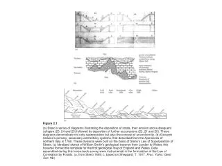
Figure 2.1 (a) Steno’s series of diagrams illustrating the deposition of strata, their erosion and subsequent collapse (25, 24 and 23) followed by deposition of further successions (22, 21 and 20). These diagrams demonstrate not only superposition but also the concept of unconformity. (b) Giovanni Arduino’s primary, secondary and tertiary systems, first described from the Apennines of northern Italy in 1760. These divisions were built on the basis of Steno’s Law of Superposition of Strata. (c) Idealized sketch of William Smith’s geological traverse from London to Wales; this traverse formed the template for the first geological map of England and Wales. Data assembled during this horse-back survey were instrumental in the formulation of the Law of Correlation by Fossils. (a, from Steno 1669; c, based on Sheppard, T. 1917. Proc. Yorks. Geol. Soc. 19.)
Figure 2.2 The main types of biozone, the operational units of a biostratigraphy. (Based on Holland 1986.)
Figure 2.3 Behavior of ideal zone and facies fossils through a hypothetical global stratigraphic section.
Figure 2.4 (a) Hypothetical and minimalist graphic correlation based on the stratigraphic distribution of the five apparent chronospecies of the Silurian brachiopod Eocoelia, in ascending order: E. hemisphaerica, E. intermedia, E. curtisi, E. sulcata and E. angelini; the first four range through the middle and upper Llandovery whereas the last is characteristic of the lower Wenlock. The ranges of these species are given from two artificial sections with the first appearances of each species plotted on both sections as x and y coordinates. The straight line fitted to the points allows a precise correlation between each part of the two sections. In this simple example all the points fit on a straight line; in practice a regression must be fitted to the scatter of data points. (b) Seriation of biostratigraphic data. The five Eocoelia species were collected from five horizons in a stratigraphic section; the data were collected and plotted randomly as a range chart. Seriation seeks to establish any structure, usually gradients, within the matrix by maximizing entries in the leading diagonal. The seriated matrix reveals the stratigraphic succession of Eocoelia species that is widely used for the correlation of Lower Silurian strata. Most seriations are based on much larger and more complex data matrices where any non-random structure, if present, is initially far from obvious.
Figure 2.4 (Continued) (c) The RASC method predicts the solution most likely to occur in the next section based on previous data. Three sections (1–3) are presented and, based on a majority vote, the RASC solution is constructed; since the first two sections are similar they win over the third slightly different section. This is different to the maximum range solution that may be constructed by other methods. (c, based on Hammer & Harper 2005.)
Figure 2.5 Approximate stratigraphic ranges through time of the main biostratigraphically useful invertebrate fossils groups. (Replotted from various sources.)
Figure 2.6 Key concepts in the definition of stratotypes and parastratotypes applicable to all stratigraphic units. The base of stage X is defined at an appropriate and suitable type section, coincident with the base of biozone Y, which can be used to correlate the base of the stage. The type section is usually conserved and further collecting across the boundary interval is restricted to the parastratotype section. The base of the stage is indicated as XXX. (Based on Temple, J.T. 1988. J Geol. Soc. Lond.145.)
Figure 2.7 Stratigraphic case study: description and definition of the litho-, bio- and chronostratigraphy of the stratotype section of the Wenlock Series, along Wenlock Edge in Shropshire, UK. This is the internationally accepted standard for the Wenlock Epoch, the third time division of the Silurian Period.
Figure 2.8 Current status of the development of a new, internationally accepted chronostratigraphy for the Ordovician System. New global series and stages are correlated with the comparable chronostratigraphic divisions used in North American and the United Kingdom and Ireland. GSSP, global standard section and point.
Figure 2.9 North American Phanerozoic sequences: the recognition of these large packages of rock or what are termed “megasequences” formed the basis for the modern discipline of sequence stratigraphy, established by the Exxon Corporation. (Based on various sources.)
Figure 2.10 Sequences, system tracts and stratigraphic surfaces defined in relation to base level and transgression–regression curves: (a) stratal architecture across a non-marine to marine transect is related to (b) sequence stratigraphies in the non-marine and marine parts of the transect. (A), positive accommodation (base level rise); BSFR, basal surface of forced regression; c.c., correlative conformity; c.u., coarsening upward; DS, depositional sequence; FR, forced regression; FSST, falling stage systems tract; f.u., fining upward; GS, genetic stratigraphic sequence; HST, highstand systems tract; IV, incised valley; LST, lowstand systems tract; MFS, maximum flooding surface; MRS, maximum regressive surface; NR, normal regression; R, ravinement surface; RST, regressive systems tract; SU, subaerial unconformity; TR, transgressive–regressive sequence; TST, transgressive systems tract. (Based on Catuneanu, O. 2002. J. African Earth Sci.35.)
Figure 2.11 DCA axis 1 sample scores plotted against the Frankfort composite section. mfs, maximum flooding surface; HST, highstand systems tract; SB/TS, combined sequence boundary and transgressive surface; TST, transgressive systems tract. (From Holland & Patzkowsky 2004.)
Figure 2.12 a) Illustration of Milankovitch frequencies showing the relationships between eccentricity, obliquity and precession cycles.
Figure 2.12(Continued) (b) Outline stratigraphy of Cenomanian Stage Upper Cretaceous chalk facies. Column 1, stages; column 2, cyclostratigraphy; column 3, sequences. (From Gale et al. 1999.)
Figure 2.13 The various methods currently available to construct the geologic time scale 2004 (GTS2004).
Figure 2.14 Carboniferous and Permian distributions of the Glossopteris flora and the Mesosaurus fauna and the fit of Gondwana. The tight fit of Gondwana and the correspondence of fossil faunas and floras across the southern continents suggested to Wegener and others that South America, Africa, India, Antarctica and Australia had drifted apart since the Permo-Triassic. (Based on Smith, P. 1990. Geoscience Canada15.)
Figure 2.15 The emergence of the Isthmus of Panama promoted the great American biotic interchange (GABI) between North and South American terrestrial vertebrates together with the radiation of the shallow-water marine benthos of the Caribbean Sea. l, litopterns; n, notoungulates. (Based on Benton 2005.)
Figure 2.16 (opposite and this page) Changing ideas on the development of the Early Paleozoic Iapetus Ocean and its faunas: (a, c, d) paleogeographic reconstructions; (b) the mobility of organisms across a closing ocean;
Figure 2.16 (Continued) (e) a cluster analysis of the Iapetus and related Early Ordovician brachiopod faunas (tinted blocks in descending order indicate low-latitude, high-latitude, low-latitude marginal and high-latitude marginal provinces);
Figure 2.16 (Continued) (f) the possible movement of the Precordilleran terrane in three stages, 1–3. A dataset of early Ordovician brachiopod distribution across the Iapetus terranes is available at http://www.blackwellpublishing.com/paleobiology/. These data may be analyzed and manipulated using a range of multivariate techniques including cluster analysis (see also Hammer & Harper 2005). (a–d, from Harper, D.A.T. 1992. Terra Nova4; f, based on Finney 2007.)
Figure 2.17 Displaced faunas in terranes within the North American Cordillera together with changing provincial boundaries on the craton. Postulated latitudinal boundaries on the craton during the Permian, Triassic and Jurassic are indicated and confirm the northern movement of these displaced terranes. A dataset of Jurassic ammonoid distributions across the cordilleran terranes is available at http://www.blackwellpublishing.com/paleobiology/. These data may be analyzed and manipulated using a range of multivariate techniques including cluster analysis (see also Hammer & Harper 2005). (From Hallam, A. 1986. J. Geol. Soc.143.)
Figure 2.18 Changing familial diversity of skeletal benthos through time in relation to plate configurations: high diversities are apparently coincident with times of greatest continental fragmentation, for example during the Ordovician, Devonian and Cretaceous-Cenozoic. A, pre-Appalachian-Variscan Ocean; H, Hispanic Corridor; I, Iapetus Ocean; U, pre-Uralian Ocean. (Based on Smith, P. 1990. Geoscience Canada15.)
Figure 2.19 Strained Cambrian trilobites from Himalaya. (Courtesy of Nigel Hughes.)
Figure 2.20 The Scandinavian Caledonides showing the pre-drift positions of some of the various thrust sheet complexes. During the Early Ordovician (EO) the most seaward, upper parts of the higher thrust sheets (Støren Nappe) contained North American marginal faunas, whereas the lower parts of these thrust sheets (Köli Nappe) contained Celtic (oceanic) type faunas. The lower parts of the nappe pile (e.g. the Valdres Nappe) have Baltic faunas. The Wenlock-Ludlow (MS) marginal molasse deposits (Old Red Sandstone (ORS) facies), for example at Ringerike, have spectacular marine marginal faunas.