Download

1 / 38
380 likes | 558 Views
A Bayesian Approach to Joint Feature Selection and Classifier Design. Balaji Krishnapuram , Alexander J. Hartemink , Lawrence Carin , Fellow, IEEE, and Mario A.T. Figueiredo , Senior Member, IEEE IEEE TRANSACTIONS ON PATTERN ANALYSIS AND MACHINE INTELLIGNEC VOL. 26, NO.9, SEPTEMBER 2004.

E N D
ABayesian Approach to Joint Feature Selection and Classifier Design BalajiKrishnapuram, Alexander J. Hartemink, Lawrence Carin, Fellow, IEEE, and Mario A.T. Figueiredo, Senior Member, IEEE IEEE TRANSACTIONS ON PATTERN ANALYSIS AND MACHINE INTELLIGNECVOL. 26, NO.9, SEPTEMBER 2004
Outline • Introduction to MAP • Introduction to Expectation-Maximization • Introduction to Generalized linear models • Introduction • Sparsity-promoting priors • MAPparameter estimation via EM • Experimental Results • Conclusion
Introduction to MAP • Maximum-likelihood estimation • is considered as parameter vector • In MAP estimation • is considered as a random vector described by a pdfp() • Assume p() is known • Given a set of training samples D={x1,x2,…,xn}
Introduction to MAP • Find the maximum of • If p() is uniform or flat enough
Introduction to generalized linear models • Supervised learning can be formalized as the problem of inferring a function y=f(x), based on a training set D={(x1,y1),…, (xn,yn)} • When y is continuous (e.g. y R ), we are in the context of regression, whereas in classification problems, y is of categorical nature (e.g. binary, y={-1,1}) • The function f is assumed to have a fixed structure and to depend on a set of parameters . • We write y=f(x, ) and the goal becomes to estimate from the training data.
Introduction to generalized linear models • Regression functionswhere is a vector of k fixed functions of the input, often called features. • Linear regression : k=d+1 • Nonlinear regression via a set of k fixed basis functions : • Kernel regression :
Introduction to generalized linear models • Assume that the output variables in the training set were contaminated by addictive white Gaussian noise :where is a set of independent zero-mean Gaussian samples with variance 2 . • With , the likelihood function : is the so-called design matrix. The element of , denoted , is given by
Introduction to generalized linear models • With a zero-mean Gaussian prior for , with covariance • The posterior is still Gaussian
Introduction to generalized linear models • In logistic regression, the link function is • Probit link or Probit model:
Introduction to generalized linear models • Hidden variable where w is a zero-mean unit-variance Gaussian noise • If the classification rule is • Given training datahidden variables where
Introduction to generalized linear models • If we had z, we would have a simple linear likelihood with unit noise variance • The use of the EM algorithm to estimate , by treating z as missing data.
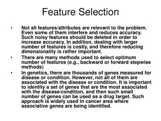
Introduction • Given the training settwo standard tasks : • Classifier design : To learn a function that most accurately predicts the class of a new example • Feature selection: To identify a subset of the features that is most informative about the class distinction (feature selection)
Introduction • In this paper, joint classifier and feature optimization (JCFO) • The association of a nonnegative scaling factor with each feature • These scaling factors are then estimated from the data, under an a priori preference for values that are either significantly large or otherwise exactly zero.
Introduction • In this paper, focus on probabilistic kernel classifiers of the form :
Introduction • two of the most popular kernels : • rth order polynomial : • Gaussian radial basis function(RBG) :
Introduction • JCFO seeks sparsity in its use of both basis functions (sparsity in ) and features (sparsity in ) • For kernel classification, sparsity in the use of basis functions is known to impact the capacity of the classifier, which controls its generalization performance. • Sparsity in feature utilization is another important factor for increased robustness.
Sparsity-promoting priors • To encourage sparsity in the estimates of the parameter vector and , we adopt a Laplacian prior for each. • For small , the difference between and is much larger for a Laplacian than for a Gaussian. • As a result, using a Laplacian prior in a learning procedure that seeks to maximize the posterior density strongly favors values of that are exactly 0 over values that are simply close to 0.
Sparsity-promoting priors • To avoid nondifferentiability at the origin, we use an alternative hierarchical formulation which is equivalent to the Laplacian prior : • Let each have a zero-mean Gaussian prior • Let all the variances be independently distributed according to a common exponential distribution (the hyperprior)
Sparsity-promoting priors • The effective prior can be obtained by marginalizing with respect to each • For each scaling coefficient , we adopt similar saprsity-promoting prior, but we must ensure that any estimate of is nonnegative.
Sparsity-promoting priors • A hierarchical model for similar to the one described above , but with the Gaussian prior replaced by a truncated Gaussian prior that explicitly forbids negative values : • An exponential hyperprior
Sparsity-promoting priors • The effective prior can be obtained by marginalizing with respect to .
MAPparameter estimation via EM • Given the priors described above, our goal is to find the maximum a posteriori (MAP) estimate :
MAPparameter estimation via EM • We use EM algorithm that finds MAP estimates using the hierarchical prior models and latent variable interpretation of the probit model. • (N+1)-dimensioanl vector function:random function :
MAPparameter estimation via EM • If a classifier were to assign the label y=1 to an example x whenever and y=0 whenever • We would recover the probit mode: • Consider the vector of missing variables:
MAPparameter estimation via EM • The EM algorithm will produce a sequence of estimates and by alternating between the E-step and the M-step. • E-step • Compute the expected value of the complete log-posterior conditioned on the data D and the current esitimateof the parameters, and .
MAPparameter estimation via EM • M-step
Experimental Results • Each data is initially normalized to have zero mean and unit variance. • The regularization parameters and (controlling the degrees of sparsity enforced on and ,respectively ) are selected by cross-validation on the training data.
Experimental Results • Effect of irrelevant predictor variables • Generate synthetic data from one of two normal distributions with unit variance
Experimental Results • Results with high-dimensional gene expression data set • Strategy for learning a classifier is likely to be less relevant here than the choice of feature selection method. • Two commonly-analyzed data sets • Contains expression level of 7129 genes from 47 patients with acute myeloid leukemia (AML) and 25 patients with acute lymphoblastic leukemia (ALL). • Contains expression levels of 2000 genes from 40 tumor and 22 normal colon tissues.
Experimental Results • Full leave-one-out cross-validation procedure: • Train on n-1 samples and test the obtained classifier on the remaining sample, and repeat this procedure for every sample.
Experimental Results • Results with low-dimensional benchmark data sets
Experimental Results • Our algorithm did not perform any feature selection in the Ripley data set, selected five out of eight variables in the Pima data set, and selected three out of five variables in the Crabs. • JCFO is also very sparse in its utilization of kernel functions: • It chooses an average of 4 out of 100, 5 out of 200, 5 out of 80, and 6 out of 300 kernels for the Ripley, Pima, Crabs, and WBC data set, respectively.
Conclusion • It use of sparsity-promoting priors that encourage many of the to be exactly zero. • Experimental results indicate that, for high-dimensional data with many irrelevant features, the classification accuracy of JCFO is likely to be statistically superior to other methods,