Feature Selection
Feature Selection. Advanced Statistical Methods in NLP Ling 572 January 24, 2012. Roadmap. Feature representations: Features in attribute-value matrices Motivation: text classification Managing features General approaches Feature selection techniques Feature scoring measures


Feature Selection
E N D
Presentation Transcript
Feature Selection Advanced Statistical Methods in NLP Ling 572 January 24, 2012
Roadmap • Feature representations: • Features in attribute-value matrices • Motivation: text classification • Managing features • General approaches • Feature selection techniques • Feature scoring measures • Alternative feature weighting • Chi-squared feature selection
Representing Input:Attribute-Value Matrix • Choosing features: • Define features – i.e. with feature templates
Representing Input:Attribute-Value Matrix • Choosing features: • Define features – i.e. with feature templates • Instantiate features
Representing Input:Attribute-Value Matrix • Choosing features: • Define features – i.e. with feature templates • Instantiate features • Perform dimensionality reduction
Representing Input:Attribute-Value Matrix • Choosing features: • Define features – i.e. with feature templates • Instantiate features • Perform dimensionality reduction • Weighting features: increase/decrease feature import
Representing Input:Attribute-Value Matrix • Choosing features: • Define features – i.e. with feature templates • Instantiate features • Perform dimensionality reduction • Weighting features: increase/decrease feature import • Global feature weighting: weight whole column • Local feature weighting: weight cell, conditions
Feature Selection Example • Task: Text classification • Feature template definition:
Feature Selection Example • Task: Text classification • Feature template definition: • Word – just one template • Feature instantiation:
Feature Selection Example • Task: Text classification • Feature template definition: • Word – just one template • Feature instantiation: • Words from training (and test?) data • Feature selection:
Feature Selection Example • Task: Text classification • Feature template definition: • Word – just one template • Feature instantiation: • Words from training (and test?) data • Feature selection: • Stopword removal: remove top K (~100) highest freq • Words like: the, a, have, is, to, for,… • Feature weighting:
Feature Selection Example • Task: Text classification • Feature template definition: • Word – just one template • Feature instantiation: • Words from training (and test?) data • Feature selection: • Stopword removal: remove top K (~100) highest freq • Words like: the, a, have, is, to, for,… • Feature weighting: • Apply tf*idf feature weighting • tf = term frequency; idf = inverse document frequency
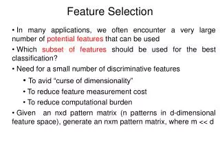
The Curse of Dimensionality • Think of the instances as vectors of features • # of features = # of dimensions
The Curse of Dimensionality • Think of the instances as vectors of features • # of features = # of dimensions • Number of features potentially enormous • # words in corpus continues to increase w/corpus size
The Curse of Dimensionality • Think of the instances as vectors of features • # of features = # of dimensions • Number of features potentially enormous • # words in corpus continues to increase w/corpus size • High dimensionality problematic:
The Curse of Dimensionality • Think of the instances as vectors of features • # of features = # of dimensions • Number of features potentially enormous • # words in corpus continues to increase w/corpus size • High dimensionality problematic: • Leads to data sparseness
The Curse of Dimensionality • Think of the instances as vectors of features • # of features = # of dimensions • Number of features potentially enormous • # words in corpus continues to increase w/corpus size • High dimensionality problematic: • Leads to data sparseness • Hard to create valid model • Hard to predict and generalize – think kNN
The Curse of Dimensionality • Think of the instances as vectors of features • # of features = # of dimensions • Number of features potentially enormous • # words in corpus continues to increase w/corpus size • High dimensionality problematic: • Leads to data sparseness • Hard to create valid model • Hard to predict and generalize – think kNN • Leads to high computational cost
The Curse of Dimensionality • Think of the instances as vectors of features • # of features = # of dimensions • Number of features potentially enormous • # words in corpus continues to increase w/corpus size • High dimensionality problematic: • Leads to data sparseness • Hard to create valid model • Hard to predict and generalize – think kNN • Leads to high computational cost • Leads to difficulty with estimation/learning • More dimensions more samples needed to learn model
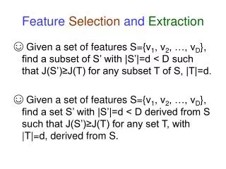
Breaking the Curse • Dimensionality reduction: • Produce a representation with fewer dimensions • But with comparable performance
Breaking the Curse • Dimensionality reduction: • Produce a representation with fewer dimensions • But with comparable performance • More formally, given an original feature set r, • Create a new set r’ |r’| < |r|, with comparable perf.
Breaking the Curse • Dimensionality reduction: • Produce a representation with fewer dimensions • But with comparable performance • More formally, given an original feature set r, • Create a new set r’ |r’| < |r|, with comparable perf. • Functionally, • Many ML algorithms do not scale well
Breaking the Curse • Dimensionality reduction: • Produce a representation with fewer dimensions • But with comparable performance • More formally, given an original feature set r, • Create a new set r’ |r’| < |r|, with comparable perf. • Functionally, • Many ML algorithms do not scale well • Expensive: Training cost, training cost • Poor prediction: overfitting, sparseness
Dimensionality Reduction • Given an initial feature set r, • Create a feature set r’ s.t. |r| < |r’| • Approaches:
Dimensionality Reduction • Given an initial feature set r, • Create a feature set r’ s.t. |r| < |r’| • Approaches: • r’: same for all classes (aka global), vs • r’: different for each class (aka local)
Dimensionality Reduction • Given an initial feature set r, • Create a feature set r’ s.t. |r| < |r’| • Approaches: • r’: same for all classes (aka global), vs • r’: different for each class (aka local) • Feature selection/filtering, vs • Feature mapping (aka extraction)
Feature Selection • Feature selection: • r’ is a subset of r • How can we pick features?
Feature Selection • Feature selection: • r’ is a subset of r • How can we pick features? • Extrinsic ‘wrapper’ approaches:
Feature Selection • Feature selection: • r’ is a subset of r • How can we pick features? • Extrinsic ‘wrapper’ approaches: • For each subset of features: • Build, evaluate classifier for some task • Pick subset of features with best performance
Feature Selection • Feature selection: • r’ is a subset of r • How can we pick features? • Extrinsic ‘wrapper’ approaches: • For each subset of features: • Build, evaluate classifier for some task • Pick subset of features with best performance • Intrinsic ‘filtering’ methods: • Use some intrinsic (statistical?) measure • Pick features with highest scores
Feature Selection • Wrapper approach: • Pros:
Feature Selection • Wrapper approach: • Pros: • Easy to understand, implement • Clear relationship b/t selected features and task perf. • Cons:
Feature Selection • Wrapper approach: • Pros: • Easy to understand, implement • Clear relationship b/t selected features and task perf. • Cons: • Computationally intractable: 2|r’|*(training + testing) • Specific to task, classifier; ad-hov • Filtering approach: • Pros
Feature Selection • Wrapper approach: • Pros: • Easy to understand, implement • Clear relationship b/t selected features and task perf. • Cons: • Computationally intractable: 2|r’|*(training + testing) • Specific to task, classifier; ad-hov • Filtering approach: • Pros: theoretical basis, less task, classifier specific • Cons:
Feature Selection • Wrapper approach: • Pros: • Easy to understand, implement • Clear relationship b/t selected features and task perf. • Cons: • Computationally intractable: 2|r’|*(training + testing) • Specific to task, classifier; ad-hov • Filtering approach: • Pros: theoretical basis, less task, classifier specific • Cons: Doesn’t always boost task performance
Feature Mapping • Feature mapping (extraction) approaches • Features r’ representation combinations/transformations of features in r
Feature Mapping • Feature mapping (extraction) approaches • Features r’ representation combinations/transformations of features in r • Example: many words near-synonyms, but treated as unrelated
Feature Mapping • Feature mapping (extraction) approaches • Features r’ representation combinations/transformations of features in r • Example: many words near-synonyms, but treated as unrelated • Map to new concept representing all • big, large, huge, gigantic, enormous concept of ‘bigness’ • Examples:
Feature Mapping • Feature mapping (extraction) approaches • Features r’ representation combinations/transformations of features in r • Example: many words near-synonyms, but treated as unrelated • Map to new concept representing all • big, large, huge, gigantic, enormous concept of ‘bigness’ • Examples: • Term classes: e.g. class-based n-grams • Derived from term clusters
Feature Mapping • Feature mapping (extraction) approaches • Features r’ representation combinations/transformations of features in r • Example: many words near-synonyms, but treated as unrelated • Map to new concept representing all • big, large, huge, gigantic, enormous concept of ‘bigness’ • Examples: • Term classes: e.g. class-based n-grams • Derived from term clusters • Dimensions in • Latent Semantic Analysis (LSA/LSI) • Result of Singular Value Decomposition (SVD) on matrix • Produces ‘closest’ rank r’ approximation of original
Feature Mapping • Pros:
Feature Mapping • Pros: • Data-driven • Theoretical basis – guarantees on matrix similarity • Not bound by initial feature space • Cons:
Feature Mapping • Pros: • Data-driven • Theoretical basis – guarantees on matrix similarity • Not bound by initial feature space • Cons: • Some ad-hoc factors: • e.g. # of dimensions • Resulting feature space can be hard to interpret
Feature Filtering • Filtering approaches: • Applying some scoring methods to features to rank their informativeness or importance w.r.t. some class
Feature Filtering • Filtering approaches: • Applying some scoring methods to features to rank their informativeness or importance w.r.t. some class • Fairly fast and classifier-independent
Feature Filtering • Filtering approaches: • Applying some scoring methods to features to rank their informativeness or importance w.r.t. some class • Fairly fast and classifier-independent • Many different measures: • Mutual information • Information gain • Chi-squared • etc…
Basic Notation, Distributions • Assume binary representation of terms, classes • tk: term in T; ci: class in C
Basic Notation, Distributions • Assume binary representation of terms, classes • tk: term in T; ci: class in C • P(tk): proportion of documents in which tk appears • P(ci): proportion of documents of class ci • Binary so have
Basic Notation, Distributions • Assume binary representation of terms, classes • tk: term in T; ci: class in C • P(tk): proportion of documents in which tk appears • P(ci): proportion of documents of class ci • Binary so have