DISCRIMINANT FUNCTION ANALYSIS (DFA)
Learn about Discriminant Function Analysis (DFA) for categorical variables and how it differs from linear regression. Understand the assumptions, purposes, and applications of DFA in analyzing and classifying groups based on attributes.

DISCRIMINANT FUNCTION ANALYSIS (DFA)
E N D
Presentation Transcript
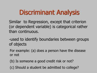
DISCRIMINANT FUNCTION ANALYSIS • DFA undertakes the same task as multiple linear regression by predicting an outcome. • Multiple linear regression is limited to cases where the DV (Y axis) is an interval variable so that estimated mean population numerical Y values are produced for given values of weighted combinations of IV (X axis) values. • But many interesting variables are categorical, such as political party voting intention, migrant/non-migrant status, making a profit or not, holding a particular credit card, owning, renting or paying a mortgage for a house, employed/unemployed, satisfied versus dissatisfied employees, which customers are likely to buy a product or not buy, what distinguishes Stellar Bean clients from Gloria Beans clients, whether a person is a credit risk or not, etc.
DISCRIMINANT FUNCTION ANALYSIS • DFA is used when • the dependent is categorical with the predictor IV’s at interval level like age, income, attitudes, perceptions, and years of education although dummy variables can be used as predictors as in multiple regression (cf. Logistic Regression where IV’s can be of any level of measurement). • there are two ormore DV categories unlike logistic regression which is limited to a dichotomous dependent variable.
ASSUMPTIONS OF DFA • Observations are a random sample. • Each predictor variable is normally distributed or approximately so. • There must be two or more mutually exclusive and collectively exhaustive groups or categories, i.e each case belongs to only one group. • Each group or category must be well defined, clearly differentiated from any other group(s). A median split on an attitude scale is not a natural way to form groups. Partitioning quantitative variables is only justifiable if there are easily identifiable gaps at the points of division, for instance employees in three salary band groups. • The groups or categories should be defined before collecting the data. • Group sizes of the DV should not be grossly different and should be at least five times the number of independent variables.
PURPOSES OF DFA • To investigate differences between groups on the basis of the attributes of the cases, indicating which attribute(s) contribute most to group separation. The descriptive technique successively identifies the linear combination of attributes known as canonical discriminant functions (equations) which contribute maximally to group separation. • Predictive DFA addresses the question of how to assign new cases to groups. The DFA function uses a person’s scores on the predictor variables to predict the category to which the individual belongs. • To classify cases into groups. Statistical significance tests using chi square enable you to see how well the function separates the groups. • To test theory whether cases are classified as predicted.
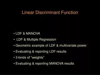
DISCRIMINANT FUNCTION ANALYSIS DFA involves the determination of a linear equation like regression that will predict which group each case belongs to. The form of the equation or canonical discriminant function is: D = v1X1 + v2X2 + v3X3 + ……..viXi + a Where D = discriminant function v = the discriminant coefficient or weight for that variable X = respondent’s score for that variable a = a constant i = the number of predictor variables
DISCRIMINANT FUNCTION ANALYSIS • This equation is like a regression equation or function. • The v’s are unstandardized discriminant coefficients analogous to the b’s in the regression equation. These v’s maximize the distance between the means of the criterion (dependent) variable. Standardized discriminant coefficients can also be used like beta weight in regression. Good predictors tend to have large weights. • This function maximizes the distance between the categories, i.e. come up with an equation that has strong discriminatory power between groups. • After using an existing set of data to calculate the discriminant function and classify cases, any new cases can then be classified. • The number of discriminant functions is one less the number of DV groups. There is only one function for the basic two group discriminant analysis.
DISCRIMINANT FUNCTION ANALYSIS • At the end of the DFA process, each group should have a normal distribution of discriminant scores. The degree of overlap between the discriminant score distributions can be used as a measure of the success of the technique
DISCRIMINANT FUNCTION ANALYSIS • In a two-group situation predicted membership is calculated by first producing a score for D for each case using the discriminate function. • Cases with D values smaller than the cut-off value are classified as belonging to one group while those with values larger are classified into the other group. SPSS will save the predicted group membership and D scores as new variables. • The group centroid is the mean value of the discriminant scores for a given category of the dependent variable. There are as many centroids as there are groups or categories. The cut-off is the mean of the two centroids. If the discriminant score of the function is less than or equal to the cut-off the case is classed as 0 whereas if it is above it is classed as 1.
SPSS EXAMPLE • This example of DFA uses demographic data and scores on various questionnaires. • ‘smoke’ is a nominal variable indicating whether the employee smoked or not. • The other variables to be used are age, days absent sick from work last year, self-concept score, anxiety score and attitudes to anti smoking at work score. • The aim of the analysis is to determine whether these variables will discriminate between those who smoke and those who do not.
SPSS EXAMPLE • 1. Analyse > Classify > Discriminant • 2. Select ‘smoke’ as your grouping variable and enter it into the Grouping Variable Box
SPSS EXAMPLE • 3. Click Define Range button and enter the lowest and highest code for your groups (here it is 1 and 2)
SPSS EXAMPLE • 4. Click Continue • 5. Select your predictors (IV’s) and enter into Independents box. Select Enter Independents Together. If you planned a stepwise analysis you would at this point select Use Stepwise Method and not the previous instruction.
SPSS EXAMPLE • Click on Statisticsbutton and select Means, Univariate Anovas, Box’s M, Unstandardized andWithin-Groups Correlation
SPSS EXAMPLE • 7. Click Continue and then Classify. Select Compute From Group Sizes, Summary Table, Leave One Out Classification, Within Groups, and allPlots
SPSS EXAMPLE • 8. Continue then Save and select Predicted Group MembershipandDiscriminant Scores. • 10. Click OK
Interpreting The Printout • The initial case processing summary as usual indicates sample size and any missing data. • Group Statistics Tables. In discriminant analysis, we are trying to predict a group membership so firstly we examine whether there are any significant differences between groups on each of the independent variables using group means and ANOVA results data. • The Group Statistics and Tests of Equality of Group Means tables provide this information. If there are no significant group differences it is not worthwhile proceeding any further with the analysis. • The next two tables provide evidence of significant differences between means of smoke and no smoke groups for all IV’s. The Pooled Within-Group Matrices also supports use of these IV’s as intercorrelations are low.
SPSS EXAMPLE Tests of Equality of Group Means Wilks' Lambda F df1 df2 Sig. age .980 8.781 1 436 .003 self concept score .526 392.672 1 436 .000 anxiety score .666 218.439 1 436 .000 Days absent last year .931 32.109 1 436 .000 total anti-smoking .887 55.295 1 436 .000 policies subtest B
SPSS EXAMPLE Pooled Within-Groups Matrices total anti-smoking self concept days absent policies age score anxiety score last year subtest B Correlation age 1.000 -.118 .060 .042 .061 self concept score -.118 1.000 .042 -.143 -.044 anxiety score .060 .042 1.000 .118 .137 .042 -.143 .118 1.000 .116 days absent last year total anti-smoking .061 -.044 .137 .116 1.000 policies subtest B
SPSS EXAMPLE • In ANOVA, an assumption is that the variances were equivalent for each group but in DFA the basic assumption is that the variance-co-variance matrices are equivalent. • Box’s M tests the null hypothesis that the covariance matrices do not differ between groups formed by the dependent. The null hypothesis is retained if the groups do not differ significantly. • Box’s M is 176.474 with F = 11.615 which is significant at p<.000. However, with large samples, a significant result is not regarded as too important. Where three or more groups exist, and M is significant, groups with very small log determinants should be deleted from the analysis
Table of eigenvalues • This provides information on each of the discriminate functions(equations) produced. • The maximum number of discriminant functions produced is the number of groups minus 1. We are using only two groups here, viz ‘smoke’ and ‘no smoke’, so only 1 function is displayed. • The canonical correlation is the multiple correlation between the predictors and the discriminant function. With only one function it provides an index of overall model fit which is interpreted as being proportion of variance explained (R2). • In our example a canonical correlation of 0.802 suggests the model explains 64.32% of the variation in the grouping variable, i.e. whether a respondent smokes or not.
Wilks’ lambda • This table indicates the proportion of total variability not explained, i.e. it is the converse of the squared canonical correlation. 35.6% is unexplained.
Standardized Canonical Discriminant Function Coefficients table • This provides an index of the importance of each predictor (cf standardized regression coefficients or beta’s in multiple regression). The sign indicates the direction of the relationship. • Self concept score was the strongest while low anxiety (note –ve sign) was next in importance as a predictor. • These two variables stand out as those that predict allocation to the smoke or do not smoke group. Age, absence from work and anti-smoking attitude score were less successful as predictors.
The structure matrix table • This provides another way of indicating the relative importance of the predictors and it can be seen below that the same pattern holds. Many researchers use the structure matrix correlations because they are considered more accurate than the Standardized Canonical Discriminant Function Coefficients. • The structure matrix table shows the correlations of each variable with each discriminate function. These Pearson coefficients are structure coefficients or discriminant loadings. They serve like factor loadings in factor analysis. By identifying the largest loadings for each discriminate function the researcher gains insight into how to name each function.
The structure matrix table • Here we have self concept and anxiety (low scores) which suggest a label of personal confidence /effectiveness as the function that discriminates between non smokers and smokers. Just like factor loadings 0.30 is seen as the cut-off between important and less important variables. • Absence and age are clearly not loaded on the discriminant function, i.e. are weakest predictors.
STRUCTURE MATRIX TABLE Structure Matrix Function 1 self concept score .706 anxiety score -.527 total anti-smoking .265 policies subtest B days absent last year -.202 age .106 Pooled within-groups correlations between discriminating variables and standardized canonical discriminant functions Variables ordered by absolute size of correlation within function.
Canonical Discriminant Function Coefficient Table • These unstandardized coefficients (b) are used to create the discriminant function (equation). It operates just like a regression equation. In this case we have: • D = (.024 x age) + (.080 x self concept ) + ( -.100 x anxiety) + ( -.012 days absent) + (.134 anti smoking score) - 4.543 • The discriminant function coefficients b indicate the partial contribution of each variable to the discriminate function controlling for all other variables in the equation. They can be used to assess each IV’s unique contribution to the discriminate function and therefore provide information on the relative importance of each variable. • If there are any dummy variables as in regression, dummy variables must be assessed as a group through hierarchical DA running the analysis first without the dummy variables then with them. The difference in squared canonical correlation indicates the explanatory effect of the set of dummy variables.
Group Centroids table • The table displays the average discriminant score for each group. In our example, non-smokers have a mean of 1.125 while smokers produce a mean of -1.598. Cases with scores near to a centroid are predicted as belonging to that group. This data is another way of viewing the effectiveness of the discrimination.
Classification Table • The classification table is one in which rows are the observed categories of the DV and columns are the predicted categories. • With perfect prediction all cases lie on the diagonal. The percentage of cases on the diagonal is the percentage of correct classifications . • The cross-validated set of data is a more honest presentation of the power of the discriminant function than that provided by the original classifications and often produces a poorer outcome. • The cross-validation is often termed a ‘jack-knife’ classification in that it successively classifies all cases but one to develop a discriminant function and then categorizes the case that was left out. This process is repeated with each case left out in turn. This cross validation produces a more reliable function. The argument behind it is that one should not use the case you are trying to predict as part of the categorization process.
CLASSIFICATION TABLE • The classification results reveal that 91.8% of respondents were classified correctly into ‘smoke’ or ‘do not smoke’ groups. • This overall predictive accuracy of the discriminant function is called the ‘hit ratio’. Non smokers were classified with slightly better accuracy (92.6%) than smokers (90.6%). • What is an acceptable hit ratio? You must compare the calculated hit ratio with what you could achieve by chance. If two samples are equal in size then you have a 50/50 chance anyway. Most researchers would accept a hit ratio that is 25% larger than that due to chance.
b,c Classification Results Predicted Group Membership smoke or not non-smoker smoker Total Original Count non-smoker 238 19 257 smoker 17 164 181 % non-smoker 92.6 7.4 100.0 smoker 9.4 90.6 100.0 a Cross-validated Count non-smoker 238 19 257 smoker 17 164 181 % non-smoker 92.6 7.4 100.0 smoker 9.4 90.6 100.0 a. Cross-validation is done only for those cases in the analysis. In cross- validation, each case is classified by the functions derived from all cases other than that case. b. 91.8% of original grouped cases correctly classified. c. 91.8% of cross-validated grouped cases correctly classified. CLASSIFICATION TABLE
Saved variables • As a result of asking the analysis to save the new groupings, two new variables can now be found at the end of your data file. • dis_1 is the predicted grouping based on the discriminant analysis coded 1 and 2, • dis1_1 are the D scores by which the cases were coded into their categories. • The average D scores for each group are of course the group centroids reported earlier. While these scores and groups can be used for other analyses, they are useful as visual demonstrations of the effectiveness of the discriminant function. As an example, histograms and box plots are alternative ways of illustrating the distribution of the discriminant function scores for each group. These are shown below and reveal very minimal overlap in the graphs and box plots; a substantial discrimination is revealed. suggesting the function does discriminate well as previous tables indicated.
NEW CASES – MAHALANOBIS DISTANCES • Mahalanobis distances (obtained from the Method Dialogue Box) are used to analyse cases as it is the measure distance between a case and the centroid for each group of the dependent. • So a new case or cases can be compared with an existing set of cases. A new case will have one distance for each group and therefore can be classified as belonging to the group for which its distance is smallest. • Mahalanobis distance is measured in terms of SD from the centroid, therefore a case that is more than 1.96 Mahalanobis distance units from the centroid has less than 5% chance of belonging to that group.
Stepwise Discriminant Analysis • Stepwise discriminate analysis, like its parallel in multiple regression, is an attempt to find the best set of predictors. • It is often used in an exploratory situation to identify those variables from among a larger number that might be used later in a more rigorous theoretically driven study. • In stepwise DA, the most correlated independent is entered first by the stepwise programme, then the second until an additional dependent adds no significant amount to the canonical R squared. The criteria for adding or removing is typically the setting of a critical significance level for ‘F to remove’
Stepwise Discriminant Analysis • We will use the same file as above. On this occasion we will enter the same predictor variables one step at a time to see which combinations are the best set of predictors or whether all of them are retained. • Only one of the SPSS screen shots will be displayed as the others are the same as those used above.
Stepwise Discriminant Analysis • Click Continue then select predictors and enter into Independentsbox . Then click on Use Stepwise Methods. This is the important difference from the previous example
Interpretation Of Printout • Many of the tables in stepwise discriminant analysis are the same as those for the basic analysis and we will therefore only comment on the extra stepwise statistics tables. • The Stepwise Statistics Table shows that 4 steps were taken with each one including another variable and therefore these 4 were included in the Variables in the Analysis and Wilks Lambda tables because each was adding some predictive power to the function. • In some stepwise analyses only the first one or two steps might be taken even though there are more variables because succeeding additional variables are not adding to the predictive power of the discriminant function.
Wilks’ Lambda table • This table reveals that all the predictors add some predictive power to the discriminant function as all are significant with p<.000.