Matplotlib
Matplotlib is a powerful 2D plotting library that allows for creating publication-quality figures in various formats and environments. It can be used in Python scripts, IPython shell, web servers, and GUI toolkits.

Matplotlib
E N D
Presentation Transcript
Matplotlib http://matplotlib.sourceforge.net/ • A python 2D plotting library • Publication quality figures in several hardcopy formats and interactive environments across platforms • Can be used in • Python scripts, • the Python and IPython shell (a la matlab or mathematica), • web application servers, and • 6 GUI toolkits • Toolkits (4) http://matplotlib.sourceforge.net/users/toolkits.html • E.g., Basemap plots data on map projections (with continental and political boundaries)
Installation • In the Matplotlib homepage, click on the download link • In the download page, click matplotlib-1.3.0.win32-py2.7.exe • Download and install • Under C:\Python26\Lib\site-packages, 2 new folders matplotlib mpl_toolkits
To test, in the Python command line, • type the 1st example (3 lines plotting a straight line) in the Tutorial (see below) • plot() creates an object and outputs info on it • Not an error report • show() displays a figure • Close it to return from the command
Documentation • Documentation page (links): http://matplotlib.org/contents.html • PyplotTutorial (8 pp.) http://matplotlib.sourceforge.net/users/pyplot_tutorial.html • User’s Guide http://matplotlib.org/users/ • Refer to as needed • Cookbook / Matplotlib http://matplotlib.org/api/cbook_api.html • Lots of good examples • Shows figure, link to page giving code and explanation
Cyrille Rossant, Learning IPython for Interactive Computing and Data Visualization, Packt Publishing, 2013, 138 pages • Amazon $27, 4.5 on 8 reviews • matplotlib FAQ http://matplotlib.sourceforge.net/faq/index.html • Using matplotlib in a python shell http://matplotlib.sourceforge.net/users/shell.html • For performance, by default, matplotlib defers drawing until the end of the • But, to test things out interactively (in the shell), usually want to update after every command • Shows how to do this • Do it with IPython
Examples http://matplotlib.org/examples/ • Just names under headings, but names are descriptive • The “What's new” page http://matplotlib.org/users/whats_new.html • Every feature ever introduced into matplotlib is listed here under the version that introduced it • Often with a link to an example or documentation • Global Module Index: http://matplotlib.org/py-modindex.html • Documentation on the various modules • This and the next 2 are comprehensive • The Matplotlib API: http://matplotlib.sourceforge.net/api/ • Documentation on the various packages • Pyplot documentation (142 pp.): http://matplotlib.org/api/pyplot_api.html
IPython http://ipython.org • Enhanced Python shell for efficient interactive work • Library to build customized interactive environments using Python • System for interactive distributed and parallel computing • “Python Programming Environments: IPython,” UC Davis http://csc.ucdavis.edu/~chaos/courses/nlp/Software/iPython.html • Simple introduction and some links
Installation and Documentation • Under Windows, IPython needs PyReadline to support color, tab completion, etc. http://ipython.org/pyreadline.html • Download the installer: follow the link and download and run pyreadline-1.7.1.win32.exe • For IPython itself, go to the download page (http://ipython.org/download.html) and click the link for the binary Windows installer for Python 2 • The documentation page (http://ipython.org/documentation.html) has links to the manual and lots of other documentation
matplotlib.pyplot vs. pylab • Package matplotlib.pyplot provides a MATLAB-like plotting framework • Package pylab combines pyplot with NumPy into a single namespace • Convenient for interactive work • For programming, it’s recommended that the namespaces be kept separate • See such things as import pylab • Or import matplotlib.pyplot as plt • The standard alias import numpy as np • The standard alias
Also from pylab import * • Or from matplotlib.pyplot import * from numpy import * • We’ll use from pylab import * • Some examples don’t show this—just assume it
Batch and Interactive Use • In a script, • import the names in the pylab namespace • then list the commands Example: file E:\SomeFolder\mpl1.py from pylab import * plot([1,2,3,4]) show() • Executing E:\SomeFolder>mpl1.py produces the figure shown • The command line hangs until the figure is dismissed (click ‘X’ in the upper right)
plot() • Given a single list or array, plot() assumes it’s a vector of y-values • Automatically generates an x vector of the same length with consecutive integers beginning with 0 • Here [0,1,2,3] • To override default behavior, supply the x data: plot(x,y) where x and y have equal lengths show() • Should be called at most once per script • Last line of the script • Then the GUI takes control, rendering the figure
In place of show(), can save the figure to with, say, savefig('fig1.png') • Saved in the same folder as the script • Override this with a full pathname as argument—e.g., savefig('E:\\SomeOtherFolder\\fig1.png') • Supported formats: emf, eps, pdf, png, ps, raw, rgba, svg, svgz • If no extension specified, defaults to .png
Matplotlib from the Shell • Using matplotlib in the shell, we see the objects produced >>> from pylab import * >>> plot([1,2,3,4]) [<matplotlib.lines.Line2D object at 0x01A3EF30>] >>> show() • Hangs until the figure is dismissed or close() issued • show() clears the figure: issuing it again has no result • If you construct another figure, show() displays it without hanging
draw() • Clear the current figure and initialize a blank figure without hanging or displaying anything • Results of subsequent commands added to the figure >>> draw() >>> plot([1,2,3]) [<matplotlib.lines.Line2D object at 0x01C4B6B0>] >>> plot([1,2,3],[0,1,2]) [<matplotlib.lines.Line2D object at 0x01D28330>] • Shows 2 lines on the figure after show()is invoked • Use close() to dismiss the figure and clear it • clf() clears the figure (also deletes the white background) without dismissing it • Figures saved using savefig() in the shell by default are saved in C:\Python27 • Override this by giving a full pathname
Interactive Mode • In interactive mode, objects are displayed as soon as they’re created • Use ion() to turn on interactive mode, ioff() to turn it off Example • Import the pylab namespace, turn on interactive mode and plot a line >>> from pylab import * >>> ion() >>> plot([1,2,3,4]) [<matplotlib.lines.Line2D object at 0x02694A10>] • A figure appears with this line on it • The command line doesn’t hang • Plot another line >>> plot([4,3,2,1]) [<matplotlib.lines.Line2D object at 0x00D68C30>] • This line is shown on the figure as soon as the command is issued
Turn off interactive mode and plot another line >>> ioff() >>> plot([3,2.5,2,1.5]) [<matplotlib.lines.Line2D object at 0x00D09090>] • The figure remains unchanged—no new line • Update the figure >>> show() • The figure now has all 3 lines • The command line is hung until the figure is dismissed
Matplotlib in IPython • Recommended way to use matplotlib interactively is with ipython • In the IPython drop-down menu, select pylab
IPython’s pylab mode detects the matplotlibrc file • Makes the right settings to run matplotlib with your GUI of choice in interactive mode using threading • IPython in pylab mode knows enough about matplotlib internals to make all the right settings • Plots items as they’re produce without draw() or show() • Default folder for saving figures on file C:\Documents and Settings\current user
More Curve Plotting • plot() has a format string argument specifying the color and line type • Goes after the y argument (whether or not there’s an x argument) • Can specify one or the other or concatenate a color string with a line style string in either order • Default format string is 'b-' ( solid blue line) • Some color abbreviations b (blue), g (green), r (red), k (black), c (cyan) • Can specify colors in many other ways (e.g., RGB triples) • Some line styles that fill in the line between the specified points - (solid line), -- (dashed line), -. (dash-dot line), : (dotted line) • Some line styles that don’t fill in the line between the specified point o (circles), + (plus symbols), x (crosses), D (diamond symbols) • For a complete list of line styles and format strings, http://matplotlib.sourceforge.net/api/pyplot_api.html#module-matplotlib.pyplot • Look under matplotlib.pyplot.plot()
The axis() command takes a list [xmin, xmax, ymin, ymax] and specifies the view port of the axes Example In [1]: plot([1,2,3,4], [1,4,9,16], 'ro') Out[1]: [<matplotlib.lines.Line2D object at 0x034579D0>] In [2]: axis([0, 6, 0, 20]) Out[2]: [0, 6, 0, 20]
Generally work with arrays, not lists • All sequences are converted to NumPy arrays internally • plot() can draw more than one line at a time • Put the (1-3) arguments for one line in the figure • Then the (1-3) arguments for the next line • And so on • Can’t have 2 lines in succession specified just by their y arguments • matplotlib couldn’t tell whether it’s • a ythen the next yor • an xthen the corresponding y • The example (next slide) illustrates plotting several lines with different format styles in one command using arrays
In [1]: t = arange(0.0, 5.2, 0.2) In [2]: plot(t, t, t, t**2, 'rs', t, t**3, 'g^') Out[2]: [<matplotlib.lines.Line2D object at 0x02A6D410>, <matplotlib.lines.Line2D object at 0x02A6D650>, <matplotlib.lines.Line2D object at 0x02A6D8D0>]
Lines you encounter are instances of the Line2D class • Instances have the following properties alpha = 0.0 is complete transparency, alpha = 1.0 is complete opacity
One of 3 ways to set line properties: Use keyword line properties as keyword arguments—e.g., plot(x, y, linewidth=2.0) • Another way: Use the setter methods of the Line2Dinstance • For every property prop, there’s a set_prop() method that takes an update value for that property • To use this, note that plot() returns a list of lines • The following has 1 line with tuple unpacking line, = plot(x, y, 'o') line.set_antialiased(False)
The 3rd (and final) way to set line properties: use function setp() • 1st argument can be an object or sequence of objects • The rest are keyword arguments updating the object’s (or objects’) properties • E.g., lines = plot(x1, y1, x2, y2) setp(lines, color='r', linewidth=2.0)
Text • The text commands are self-explanatory • xlabel() • ylabel() • title() • text() • In simple cases, all but text() take just a string argument • text() needs at least 3 arguments: x and y coordinates (as per the axes) and a string • All take optional keyword arguments or dictionaries to specify the font properties • They return instances of class Text
plot([1,2,3]) xlabel('time') ylabel('volts') title('A line') text(0.5, 2.5, 'Hello world!')
Three ways to specify font properties: using • setp • object oriented methods (We skip this) • font dictionaries • Use setp to set any property t = xlabel('time') setp(t, color='r', fontweight='bold') • Also works with a list of text instances—e.g., labels = getp(gca(), 'xticklabels') setp(labels, color='r', fontweight='bold')
All text commands take an optional dictionary argument and keyword arguments to control font properties • E.g., to set a default font theme and override individual properties for given text commands font = {'fontname' : 'Courier', 'color' : 'r', 'fontweight' : 'bold', 'fontsize' : 11} plot([1,2,3]) title('A title', font, fontsize=12) text(0.5, 2.5, 'a line', font, color='k') xlabel('time (s)', font) ylabel('voltage (mV)', font)
Legends • A legend is a box (by default in upper right) associating labels with lines (displayed as per their formats) legend(lines, labels) where lines is a tuple of lines, labels a tuple of corresponding strings from pylab import * lines = plot([1,2,3],'b-',[0,1,2],'r--') legend(lines, ('First','Second')) savefig('legend')
If there’s only 1 line, be sure to include the commas in the tuples lengend((line1,), ('Profit',)) • Use keyword argument loc to override the default location • Use predefined strings or integer codes ‘upper right’ 1 ‘upper left’ 2 ‘lower left’ 3 ‘lower right’ 4 ‘right’ 5 ‘center left’ 6 ‘center right’ 7 ‘lower center’ 8 ‘upper center’ 9 ‘center’ 10 • E.g., legend((line,), ('Profit',) , loc=2)
Bar Charts • Function bar() creates a bar chart • Most of the arguments may be either scalars or sequences • Say in […] what they normally are Required arguments left x coordinates of the left sides of the bars [sequence] height height of the bars [sequence]
Some optional keyword arguments orientation orientation of the bars (‘vertical’ | ‘horizontal’) width width of the bars [scalar] color color of the bars [scalar] xerr if not None, generates error ticks on top the bars [sequence] yerr if not None, generates errorbars on top the bars [sequence] ecolor color of any errorbar [scalar] capsize length (in points) of errorbar caps (default 2) [scalar] logFalse (default) leaves the orientation axis as is, True sets it to log scale
For the following example, need the following yticks(seq, labels) • Make the ticks on the y axis at y-values in seq with labels the corresponding elements of labels • Without labels, number as per seq xticks(seq, labels) • Same, but for the x axis xlim(xmin, xmax) • The values on the x axis go from xmin to xmax
from pylab import * labels = ["Baseline", "System"] data = [3.75, 4.75] yerror = [0.3497, 0.3108] xerror = [0.2, 0.2] xlocations = array(range(len(data)))+0.5 width = 0.5 csize = 10 ec = 'r' bar(xlocations, data, yerr=yerror, width=width, xerr=xerror, capsize=csize, ecolor=ec) yticks(range(0, 8)) xticks(xlocations+ width/2, labels) xlim(0, xlocations[-1]+width*2) title("Average Ratings on the Training Set") savefig('bar')
Histograms hist(x, bins=n ) • Computes and draws a histogram • x: a sequence of numbers (usually with many repetitions) • If keyword argument bins is an integer, it’s the number of (equally spaced) bins • Default is 10 from pylab import * import numpy x = numpy.random.normal(2, 0.5, 1000) hist(x, bins=50) savefig('my_hist')
Scatter Plots scatter(x, y) • x and y are arrays of numbers of the same length, N • Makes a scatter plot of x vs. y from pylab import * N = 20 x = 0.9*rand(N) y = 0.9*rand(N) scatter(x,y) savefig('scatter_dem')
Keyword Arguments s • If an integer, size of marks in points2 , i.e., area occupied (default 20) • If an array of length N, gives the sizes of the corresponding elements of x, y marker • Symbol marking the points (default = ‘o’) • Same options as for lines that don’t connect the dots • And a few more c • A single color or a length-N sequence of colors
from pylab import * N = 30 x = 0.9*rand(N) y = 0.9*rand(N) area = pi * (10 * rand(N))**2 # 0 to 10 point radius scatter(x,y,s=area, marker='^', c='r') savefig('scatter_demo')
Odds and EndsHorizontal and Vertical Lines hlines(y, xmin, xmax) • Draw horizontal lines at heights given by the numbers in array y • If xmin and xmax are arrays of same length as y, they give the left and right endpoints of the corresponding lines, resp. • If either is a scalar, all lines have the same endpoint, specified by it • Some keyword arguments • linewidth (or lw): line width in points • color: default ‘k’ vlines(x, ymin, ymax) is similar but for vertical lines
from pylab import * y = arange(0,3,0.1) x = 2*y hlines(y, 0, x, color='b', lw=4) savefig('hlines')
Axis Lines • axhline() draws a line on the x axis spanning the horizontal extent of the axes • axhline(y) draws such a line parallel to the x axis at height y • Some keyword arguments color: default ‘b’ label linewidth in points • axvline() is similar but w.r.t. the y axis
Grid Lines • grid(True) produces grid lines at the tick coordinates • grid(None) suppresses the grid • grid() toggles the presence of the grid • Some keyword arguments color: default ‘k’ linestyle: default ‘:’ linewidth • Some Axes instance methods get_xgridlines() get_ygridlines() • Example: setp(gca().get_xgridlines(), color='r')
Resizing the Figure • Often should make the figure wider or higher so objects aren’t cramped • Use Figure instance methods get_size_inches() and set_size_inches() • To get an array of the 2 dimensions in inches (width then height): fig = gcf() dsize = fig.get_size_inches() • E.g., to double the width fig.set_size_inches( 2 * dsize[0], dsize[1] ) • See the example in the SciPy Cookbook http://www.scipy.org/Cookbook/Matplotlib/AdjustingImageSize
Multiple Subplots • Functions axes() and subplot() both used to create axes • subplot() used more often subplot(numRows, numCols, plotNum) • Creates axes in a regular grid of axes numRows by numCols • plotNum becomes the current subplot • Subplots numbered top-down, left-to-right • 1 is the 1st number • Commas can be omitted if all numbers are single digit • Subsequent subplot() calls must be consistent on the numbers or rows and columns
subplot() returns a Subplot instance • Subplot is derived from Axes • Can call subplot() and axes() in a subplot • E.g., have multiple axes in 1 subplot • See the Tutorial for subplots sharing axis tick labels
from pylab import * subplot(221) plot([1,2,3]) subplot(222) plot([2,3,4]) subplot(223) plot([1,2,3], 'r--') subplot(224) plot([2,3,4], 'r--') subplot(221) plot([3,2,1], 'r--') savefig('subplot')