Download

1 / 36
360 likes | 477 Views
Up-to-date Longitudinal Analysis with Individual Growth Curves Warren Lambert Peabody College & Vanderbilt Kennedy Center March 2008. Intro and Readings 2. S&W Examples 3. Sibs’ Head Size Pilot 4. Jittery Mouse Movies.

E N D
Up-to-date Longitudinal Analysis with Individual Growth Curves Warren Lambert Peabody College & Vanderbilt Kennedy Center March 2008
Intro and Readings 2. S&W Examples 3. Sibs’ Head Size Pilot 4. Jittery Mouse Movies Longitudinal analysis in Ancient Times . . . Mistakes Median splits on continuous variables ANOVA instead of ANCOVA RM ANOVA not mixed model (PROC MIXED, HLM: 20 years). Individual growth curves ignored Obsession with sig. tests No confidence intervals on plot No effect sizes (Cohen 1988, due in 16 years) JPSP 1972
Intro and Readings 2. S&W Examples 3. Sibs’ Head Size Pilot 4. Jittery Mouse Movies Making charts in Ancient Times . . . JPSP 1972 Drafting: Leroy lettering device • Make table with BMD 8V Fortran program • Make “camera ready” graph with Leroy lettering guide + India ink • Photographer for “camera-ready glossies”
Intro and Readings 2. S&W Examples 3. Sibs’ Head Size Pilot 4. Jittery Mouse Movies Computing in in Ancient Times . . . 1972 • Keypunch the data & program on IBM cards at computer center. • Sort data cards with “proc sort” machine. If cards sorted wrong, answers are wrong. • Run with BMDP 8V (balanced with no missing values). • Later, pick up printout from bin.
Intro and Readings 2. S&W Examples 3. Sibs’ Head Size Pilot 4. Jittery Mouse Movies Graphics Then (JCCP 1998, 8 numbers) Graphics Now Follows Tufte & Cleveland Complex, hundreds or thousands of numbers Small multiples of tiny charts Takes time to assimilate No distracting chart junk No wasted space or ink Now Science March 2008 Business graphics Scientific graphics
Intro and Readings 2. S&W Examples 3. Sibs’ Head Size Pilot 4. Jittery Mouse Movies Getting started now If you use the mouse to run SPSS, Bickel offers concrete instructions. In this way HLM becomes “just another GLM.”
Intro and Readings 2. S&W Examples 3. Sibs’ Head Size Pilot 4. Jittery Mouse Movies Getting started now Teach yourself graphic-rich longitudinal analysis: Work through S&W chapters 1-5 using your preferred software and S&W’s: http://www.ats.ucla.edu/stat/examples/alda/ (Or Google: UCLA ALDA) ALDA: Applied Longitudinal Data Analysis PS. W&S flipped coin for first author.
Intro and Readings 2. S&W Examples 3. Sibs’ Head Size Pilot 4. Jittery Mouse Movies Getting started now http://www.ats.ucla.edu/stat/seminars/alda/default.htm Suggestion Go to this site and start the slideshow. Then start the movie to hear & watch the lecture. Advance the slides to keep up.
Intro and Readings 2. S&W Examples 3. Sibs’ Head Size Pilot 4. Jittery Mouse Movies Getting started now Work S&W’s examples in your preferred software, MPLUS, MLwiN, HLM, SAS, Stata, R, or SPSS. Use the examples & W&S book to learn longitudinal analysis. Then you’re ready for original multilevel research! KC stats consultants and biostats clinics will help P.R.N.
Intro and Readings 2. S&W Examples 3. Sibs’ Head Size Pilot 4. Jittery Mouse Movies S&W’s Methods SAS SPSS Begin with individual growth curves. Code available in many languages, including SAS, SPSS, R, and STATA. STATA R
Intro and Readings 2. S&W Examples 3. Sibs’ Head Size Pilot 4. Jittery Mouse Movies S&W’s Methods Look at individual growth curves fit with nonparametric lines After looking at the disconnected points, fit models to the points using few assumptions (e.g. Loess, smooth, spline). Are there patterns that suggest a reasonable math model?
Intro and Readings 2. S&W Examples 3. Sibs’ Head Size Pilot 4. Jittery Mouse Movies S&W’s Methods See if a linear slope-as-outcome model makes sense. Always consider a convenient linear model (“HLM”), but only use it if it is realistic, as it is in this case. Next a few outside examples.
Intro and Readings 2. S&W Examples 3. Sibs’ Head Size Pilot 4. Jittery Mouse Movies Viewing the whole sample of individual subjects is often possible. • Abused women in urban emergency room • N = 493 • Each line is a woman and each dot is reported abuse incident. • Chart shows the great range of abuse in the sample • Means could be deceiving
Intro and Readings 2. S&W Examples 3. Sibs’ Head Size Pilot 4. Jittery Mouse Movies Viewing the whole sample of individual subjects is often possible. 6 months, 7 waves, right? • Families had 7 waves over six months • We called it “monthly” • Pattern blurred by Wave 3 • Use a mixed model that likes unequal intervals 6 months 7 waves, right?
Intro and Readings 2. S&W Examples 3. Sibs’ Head Size Pilot 4. Jittery Mouse Movies Look at individual curves if you don’t know the model for time
Intro and Readings 2. S&W Examples 3. Sibs’ Head Size Pilot 4. Jittery Mouse Movies Make spaghetti charts to compare the mean curve (linear or nonlinear) with individual curves. It is quite possible that no single individual has the mean timeline. These charts can be made with code from S&W Charts help you understand the mean curve without worshipping it
Intro and Readings 2. S&W Examples 3. Sibs’ Head Size Pilot 4. Jittery Mouse Movies Systematically build up the model . . . add group by time interactions. Use likelihood ratio tests (LRTs) to see if extra terms improve model fit. Check pseudo-R2 based on r(observed, predicted) Use plots to interpret slope coefficients (time, group by time). Explain the Group by Time interaction visually.
Intro and Readings 2. S&W Examples 3. Sibs’ Head Size Pilot 4. Jittery Mouse Movies Longitudinal coefficients may need concrete explanations. Can the reader understand this?
Intro and Readings 2. S&W Examples 3. Sibs’ Head Size Pilot 4. Jittery Mouse Movies Longitudinal coefficients may need concrete explanations. • Outcome experiment’s two questions • Do groups A and B start out equal? • Do group A and B have the same slopes?
Intro and Readings 2. S&W Examples 3. Sibs’ Head Size Pilot 4. Jittery Mouse Movies Q: What does a 2-wave pre-post longitudinal analysis show?A: Not much • Outcome experiment’s two questions • Do groups A and B start out equal? • Do group A and B have the same slopes? Lambert, E. W., A. Doucette & Bickman, L. (2001). "Measuring Mental Health Outcomes with Pre-post Designs." Journal of Behavioral Health Services Research28(3): 273-286.
Intro and Readings 2. S&W Examples 3. Sibs’ Head Size Pilot 4. Jittery Mouse Movies Q: What does a 2-wave pre-post longitudinal analysis show?A: Not much Lambert, E. W., A. Doucette & Bickman, L. (2001). "Measuring Mental Health Outcomes with Pre-post Designs." Journal of Behavioral Health Services Research28(3): 273-286.
Intro and Readings 2. S&W Examples 3. Sibs’ Head Size Pilot 4. Jittery Mouse Movies Pilot Data: Head size and autism (Study ongoing, data still coming in) 1155 babies 397 have normal sib 758 have autistic sib 4160 head circumferences Many measured at 6, 12, 18, 36 months Mean min ≈ 37 cm Mean max < 52 cm Growth looks curvilinear – any suggestions?
Intro and Readings 2. S&W Examples 3. Sibs’ Head Size Pilot 4. Jittery Mouse Movies Running an HLM (hierarchical linear model) is very popular. Slope as outcome Common hierarchical linear model (HLM). Linear is easy to understand Constant growth rate of red group a little higher in cm/month. Anyone see a problem? Suggest a solution?
Intro and Readings 2. S&W Examples 3. Sibs’ Head Size Pilot 4. Jittery Mouse Movies Use age and age squared as X’s to produce a smooth quadratic curve. Linear model didn’t work because head size doesn’t keep growing at a constant rate forever Quad-time adds constant deceleration to the model. Any problem? P.S. What’s a squared month?
Intro and Readings 2. S&W Examples 3. Sibs’ Head Size Pilot 4. Jittery Mouse Movies Try a real nonlinear model The good news Exponential growth fits better and raises the hope that the parameters will mean something. What’s a “squared month?” Model ~ decelerating growth that reaches a limit (asymptote)
Intro and Readings 2. S&W Examples 3. Sibs’ Head Size Pilot 4. Jittery Mouse Movies The bad news: Nonlinear model is complicated! Circumference (age) = B0 + B1 * (1 - EXP((B2 * AGE))); FIXED EFFECTS B01 = 36.2761 /* BIRTH 36 CM */ B11 = 13.6990 /* AVERAGE GROWTH LIMIT 14 CM */ B21 = -0.1287 /* RATE OF GROWTH PER MONTH */ RANDOM EFFECTS B0 = B01 + U0 ; * *** 36 CM BIRTH SIZE (WITH SUBJECT OFFSETS) ; B1 = B11 + U1 ; * *** FIXED STARTING DELTA OF 14 CM ; B2 = B21 + U2 ; * *** GROWTH RATE PARM -0.13 PER MONTH ; The good news Conceivable that B0, B1, and B2 have biological basis
Intro and Readings 2. S&W Examples 3. Sibs’ Head Size Pilot 4. Jittery Mouse Movies Compare different models with individual animated GIFs • Longitudinal experiment with 34 repeated measures per mouse • 12 mice: 6 knockouts + 6 “wild” mice • X is minutes and Y is activity • Evaluate statistical models using each individual’s model scores & observed scores. • Do the knockouts (PV/PV) respond more to Ritalin than the normals (WT, wild type)?
Intro and Readings 2. S&W Examples 3. Sibs’ Head Size Pilot 4. Jittery Mouse Movies Compare different models with animated GIFs. Start simple. Let’s start with a two wave pre-post model Look at each individual mouse. SAS Code for animated GIF Proc gplot etc . . . . by Subject_ID ; filename MOVEgif '.\hmix1.gif'; goptions device = gifanim gsfname = MOVEgif gsfmode = replace iteration = 0 delay = 200 xpixels = 1200 ypixels = 1200 GEPILOG = '3B'x display ; Animated GIF = stack of pictures
Intro and Readings 2. S&W Examples 3. Sibs’ Head Size Pilot 4. Jittery Mouse Movies Compare different models with animated GIFs. Gradually build up. Now a 34 wave RM ANOVA. Time is categorical, not ordinal. Under compound symmetry we assume that minute 20 and minute 160 are equally close to minute 180. Assumptions not found in most situations. Nich, C. and K. Carroll (1997). "Now you see it, now you don't: A comparison of traditional versus random-effects regression models in the analysis of longitudinal follow-up data from a clinical trial." Journal of Consulting and Clinical Psychology65(2): 252-261.
Intro and Readings 2. S&W Examples 3. Sibs’ Head Size Pilot 4. Jittery Mouse Movies Compare different models with animated GIFs. Gradually build up. Two slopes fit all? Are the residuals (vertical distance from star to line) random? Are residuals balanced (over or under?) Look at the residuals in the startup interval 0-30 minutes.
Intro and Readings 2. S&W Examples 3. Sibs’ Head Size Pilot 4. Jittery Mouse Movies Compare different models with animated GIFs. Gradually build up. Assume the mouse was randomly sampled from a population (that’s my story and I’m sticking to it). Mouse is a random effect A “random intercept” gives each mouse its own personal offset up or down. These offsets, like residuals, sum to zero for the sample. Accounts for some mice being more energetic than others.
Intro and Readings 2. S&W Examples 3. Sibs’ Head Size Pilot 4. Jittery Mouse Movies Compare different models with animated GIFs. Gradually build up. We add a slope as a random effect for each individual mouse Model moves up and down and different slopes for individuals Represent characteristics each individual arrived with Are the residuals looking better?
Intro and Readings 2. S&W Examples 3. Sibs’ Head Size Pilot 4. Jittery Mouse Movies Compare different models with animated GIFs. Gradually build up. In a “hockeystick model” different time intervals have separate slopes Early slope for habituation and another slope for Ritalin A time-varying covariate marking the times when injections were given. 00001000001000001000001
Intro and Readings 2. S&W Examples 3. Sibs’ Head Size Pilot 4. Jittery Mouse Movies Which model tells a clear story?
Intro and Readings 2. S&W Examples 3. Sibs’ Head Size Pilot 4. Jittery Mouse Movies What did we get? We got a theoretically interpretable model, not a perfect fit. RM ANOVA fits pretty well, but categorical time just doesn’t make sense.
Conclusions • Individual growth curves make it possible to model time accurately. • Good longitudinal statistical models and good software are now available. Scientists who do hands-on data analysis can now do up-to-date graphic-enriched longitudinal analysis. • Good reference books are available and self-teaching is feasible with the ALDA site. • After initial practice, you can treat a mixed model as “just another regression or ANOVA.” • Multiple repeated measures are valuable, and the pre-post two-wave design is generally a bad idea (3 waves ~ truly longitudinal). • Time spent understanding the role of time is well spent. • It is now possible to show results graphically in ways that explain the role of time while demonstrating the validity of your conclusions