Download
1 / 35
350 likes | 424 Views
Biased Random Simulation Guided by Observability-Based Coverage. Serdar Tasiran Compaq Systems Research Center, formerly GSRC, UC Berkeley Farzan Fallah Fujitsu Labs of America David G. Chinnery, Scott K. Weber, Kurt Keutzer UC Berkeley. Reference model.

E N D
Biased Random Simulation Guided by Observability-Based Coverage Serdar TasiranCompaq Systems Research Center, formerly GSRC, UC BerkeleyFarzan FallahFujitsu Labs of America David G. Chinnery, Scott K. Weber, Kurt KeutzerUC Berkeley CONFIDENTIAL
Reference model Simulation-based Functional Validation Functional Validation Simulation Input stimulus generation Monitors, assertions, comparison w/ ref. model Design (RTL model)
Functional Validation Simulation Reference model Monitors, assertions, comparison w/ ref. model Design (RTL model) Simulation with Coverage Feedback Input stimulus generation Diagnosis ofunverifiedportions Coveragemeasurement and analysis
Functional Validation Reference model Monitors, assertions, comparison w/ ref. model Our Work Simulation Input stimulus generation Design (RTL model) Diagnosis ofunverifiedportions Coveragemeasurement and analysis
2 Input stimulus generation Biased-randominput generation Design (RTL model) 3 1 Tag coverage analysis(Observability-based coverage) Coverage measurement and analysis Compute new biases to target non-covered tags Our work Outline Simulation Simulation Diagnosis ofunverifiedportions
Biased-randominput generation Design under test 1 Tag coverage analysis(Observability-based coverage) Compute new biases to target non-covered tags Coverage measurement and analysis Outline Simulation Simulation
Observability Functional Validation • Simulation detects a bug only if • a monitor flags an error, or • design and reference model differ on a variable • Variables checked for functional correctness called observed variables. • Portion of design covered only when • it is exercised during simulation (controllability) • a discrepancy originating in that portion causes discrepancy in an observed variable (observability) • Low observability Þfalse sense of security • Most of the design is exercised • Looks like high coverage • But most bugs not detected by monitors or reference model • They would have been detected if inputs chosen properly Simulation Monitors, assertions, comparison w/ ref. model Reference model Design (RTL model)
Tag Coverage [Devadas, Keutzer, Ghosh ‘96] • HDL code coverage metrics+observability requirement. • Bugs modeled as errors in HDL assignments. • A buggy assignment may be stimulated, but still missed EXAMPLES: • Wrong value generated speculatively, but never used. • Wrong value is computed and stored in memory • Read 1M cycles later, but simulation doesn’t run that long.
K C D A F Tag Coverage [Devadas, Keutzer, Ghosh ‘96] • Generalization of “stuck-at” fault coverage to HDL code • Handles multi-valued variables • Error model: An HDL assignment computes a value • higher (+D) or • lower (-D) than the intended value. • Example: 3 + D represents values > 3 A+D = 3 A= 3 C= F - 2A D= K*C +D -D +D ??? -D
Tag Coverage • Run simulation vectors • Tag one variable assignment at a time • Use tag calculus • Confirms that • HDL line is activated and • its effect is propagated to an observable variable • Tag Coverage: Subset of tags that propagate to observed variables • Efficient tool: OCCOM [Fallah, et. al.] A= 3 C= F - 2A D= K*C +D -D +D ??? -D
Biased-randominput generation 2 Biased-randominput generation Design under test Coverage measurement and analysis Outline Simulation Simulation Diagnosis ofunverifiedportions Compute new biases to target non-covered tags Tag coverage analysis(Observability-based coverage)
Portion of Computation Time 100% 0% Find Simulate Rationale for Biased-Random Vector Generation • Primary inputs selected according to a probability distribution • Trade-off between • Time to find “good” vectors • Time to simulate vectors • Typically > 50% of simulation is biased random simulation • Improved random vectors Þbetter validation overall • Less intelligence for selecting next step but many more vectors • Can explore deeper into state space
Biased Random Vector Generation • Primary inputs at each clock cycle selected according to a probability distribution • Distributions can be functions of circuit state • Distributions ( “weights” ) determined prior to simulation i1 i2 i3 s1 s2 Probability Distributions (“Weights”) P(i1 = 0) = 0.7P(i1 = 1) = 0.3 P(i2 = 0 |s1 = 1) = 0.6P(i2 = 1 |s1 = 0) = 0.7 P(i3 = 0) = 0.4P(i3 = 1) = 0.6
i1 i2 i32 Why Optimize Biases? • Very unlikely to exercise certain cases with uniform random simulation P(i1 = 1) = P(i2 = 1) = … = P(i32 = 1) = 0.5Þ P(o = 1) = 2-32 ... o • Wunderlich [DAC ‘85, Int’l. Test Conf. ‘88] • Even for combinational circuits several sets of biases required for good fault coverage • Biases must be picked based on targeted tags.
Biased-randominput generation Design under test 3 Tag coverage analysis(Observability-based coverage) Coverage measurement and analysis Compute new biases to target non-covered tags Outline Simulation Simulation Diagnosis ofunverifiedportions Compute new biases to target non-covered tags
Optimizing Input Biases • Optimization algorithm determines biases based on • Set of tags targeted • A structural netlistdescribing the circuit (BLIF-MV) • Intuitive goal • Maximize expected number of tags that will be covered COVER(Circuit,Tags) repeat while (tag coverage rate) > (threshold) Biases =Optimize_Input_Biases(Circuit, Tags) Biased_Random_Simulate(Circuit, Biases), Tags = Tags - Tags_Covered
P(i=1) = 0.2 P(s0) = 0 P(s1) = 0 P(s2) = 0.25 P(s3) = 0.25 P(s4) = 0.5 Modeling Biased Random Simulation • Key subroutine for optimizing input biases: Estimate coverage for given primary input distributions. • Transition probabilities fixed at each state • Model circuit + random generation of inputs as Markov chain. • Long simulation runsÞAnalyze behavior of circuit at steady state. - Determine tag detection probability at steady state • Huge state spaceÞApproximate analysis s1 i=0 i=0 s4 s0 i=1 i=1 i=1 i=1 s3 s2 i=0 i=0
(s1,s2)= (a1,a2) s1 s2 (s’1,s’2)= (a’1,a’2) Approximation I: Line Probabilities Compute probability distributions of statevariables instead of states Prob((s1,s2) = (a1,a2))= Prob(s1=a1)x Prob(s2=a2) • Ignores correlations between latches • Devadas, et. al. [VLSI ’95] • Power estimates within 3% for benchmarks • Individual node distributions correct within 15% • Refinement: Group closely correlated state variables into a single variable.
Steady-State Fixed-point prob(ns1 = v1) = prob( f1(i1, i2, … , im, ps1, ps2, … , psn) = vi) = prob(ps1 = v1) …prob(nsi= vj) = prob( fn(i1, i2, … , im, ps1, ps2, … , psn) = vj) = prob(psi = vi) Given input probability distributions P(ns1=v1) s1 P(ps1=v1) P(ns2=v2) s2 P(ps2=v2)
P(ns1=v1) P(ps1=v1) s1 P(ns2=v2) s2 P(ps2=v2) Computing Latch PDs at Steady-State • Start with initial guess for latch PDs • Given PDs for inputs and latch outputs, compute PDs at latch inputs • Substitute new distributions at latch outputs • Repeat until convergence • Guaranteed under minor restrictions • Key computation: Propagating PDs • Given PDs at the inputs of a combinational circuit, determine PDs at each node. Given input probability distributions
i0 P(i0 = 2) P(i0 = 0) i1 i1 i1 i2 i2 1 0 Propagating probability distributions • Given probability distributions (PDs) at inputs and latch outputscompute PDs of circuit nodes • Represent each node as a function of primary inputs • Inputs assumed independent Þ Use recursive algorithm on MDD to compute node PDs
Approximation II: Clustering • While propagating probabilities forward, impose limit on MDD size. • When limit reached, treat intermediate node as primary input • Correlations outside clusters ignored. n1 i0 P(i0 = 2) P(i0 = 0) i1 i1 i1 n1 n1 1 0
f q xi p s yj r Estimating Tag Detectability • Given PDs of each circuit node, estimate controllabilityand observability of tags • Recall +D: • Actual value of node xi is q • Intended value is p • q > p Controllability: Probability that xi = p at steady state (Done) Observability: Probability that xi = q causes change in observed variable. • Function of PDs of other nodes • May happen along a multi-cycle path
f q xi p s yj r Observability Computation Observability: Probability that xi = p q causes change in observed variable. • Propagate observabilities backward, starting from observed variables • Determine observability of xi based on • observability of yj. • PDs of related circuit nodes • Form MDD representing condition for xi = p q to be observed • Compute probability that MDD evaluates to 1. • Many paths: Pick best cluster (yj)
Observability Propagation • Propagate observabilities backward, starting from observed variables • Discrepancies may take multiple cycles to reach observed variable. • Perform several backward passes of observability computation • Stop at e.g. 10 passes. Analysis too inaccurate for more passes.
Optimization Criteria • Intuitive goal of weight determination algorithm: • Maximize expected number of tags that biased random simulation will cover • Use merit and cost functions to formalize goal • For a single tag (latch): • Add merit (cost) functions for all targeted tags (latches) cost merit Deviation of latch distribution from uniform Tag detectionprobability
Optimizing Input Distributions repeat For each primary input i Select a set of probability distributions p0, p1, p2, …, pn For j=0,…,n Compute merit functions for P(i=1) = pj Pick the j that yields best merit function until no improvement in merit function
Experimental Results: s1423 Optimized biases Uniform biases
s1423 – early in simulation Optimized biases Uniform biases
Experimental Results: s5378 Optimized biases Uniform biases Second round of bias optimization starts
Circuit Tags not covered Merit fn. comp. CPU time/ iteration (s) Uniformrandom Biasedrandom s1196 74 17 1122 1 1 1 12 1 s1238 164 35 1080 10 10 3.5 281 1 sbc 28 40 2158 428 294 4 53 4 s1423 74 17 1482 370 53 13 69 4 s5378 164 35 5043 613 100 12 100 4 8085 193 18 8276 5999 5412 75 53 4 s38584 1452 12 36100 11151 10010 104 205 3 dlx 62 25 676 187 180 3 12 2 s13207 669 31 9450 2572 2560 93 270 1 s15850 597 14 13329 11259 11184 42 262 1 Memory (MB) # iterations # latches # inputs # tags
Conclusions • On some examples, significant improvement in coverage with reasonable computational cost • No manual effort required • Longer uniform random simulations do not achieve same result • Coverage feedback is a powerful tool in input vector generation. • On other examples, coverage not improved. • Hundreds of simulations with different biases show no improvement • Circuit size is not t limiting factor: • Good results on some large circuits, bad results on some small ones • Close to complete coverage on large combinational benchmarks • For examples with bad coverage, most latches show no activity. • Conjecture: Ignoring input constraints and initialization sequences cause circuits not to be driven properly
Conclusions • Biased random patterns do not provide enough controlon the simulation runfor some circuits. • Not a standalone technique. Must be used in conjunction with more powerful, deterministic methods. • ATPG, approximate reachability, … • Better biased random simulation complements other approaches
Future research directions • Current method limited to multi-valued variables with small ranges • Generalize method to larger datapaths. • Handle datapath-control interaction • Experiment with higher level RTL descriptions. • E.g., explore biased random simulation at instruction level. • Pure biased random simulation is too weak • Explore choice of state-dependent biases • Aid bias selection in randomized test programs