Partial Observability

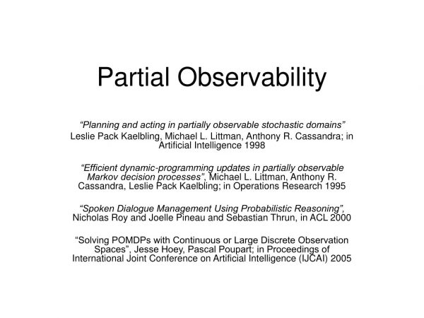
1. Partial Observability “Planning and acting in partially observable stochastic domains” Leslie Pack Kaelbling, Michael L. Littman, Anthony R. Cassandra; in Artificial Intelligence 1998 “Efficient dynamic-programming updates in partially observable Markov decision processes”, Michael L. Littman, Anthony R. Cassandra, Leslie Pack Kaelbling; in Operations Research 1995 “Spoken Dialogue Management Using Probabilistic Reasoning”, Nicholas Roy and Joelle Pineau and Sebastian Thrun, in ACL 2000 “Solving POMDPs with Continuous or Large Discrete Observation Spaces”, Jesse Hoey, Pascal Poupart; in Proceedings of International Joint Conference on Artificial Intelligence (IJCAI) 2005

2. Review of MDP

3. For MDPs we can compute the optimal policy π and use it to act by simply executing π(s) for current state s. • What happens if the agent is no longer able to determine the state it is currently in with complete reliability?

4. POMDP framework • A POMDP can be described as a tuple <S, A, T, R, Ω,O> • S, A, T, and R describe an MDP • Ω is a finite set of observations the agent can experience of its world • O:SA П(Ω) is the observation function, which gives, for each action and resulting state, a probability distribution over possible observations (we write O(s’,a,o) for the probability of making observation o given that the agent took action a and landed in state s’)

5. Problem structure • Because the agent doesn’t know the exact state, he keeps an internal belief state, b, that summarizes its previous experience. • The problem is decomposed into two parts • State estimator: update the belief state based on the last action, the current observation, and the previous belief state • The policy: maps the belief state to actions

6. An example • There are actions: EAST and WEST, each succeeds with probability 0.9, and when they fail the movement is in the opposite direction. If no movement is possible in particular direction, then the agent remains in the same location • Initially [0.33, 0.33, 0, 0.33] • After taking one EAST movement [0.1, 0.45, 0, 0.45] • After taking another EAST movement[0.1, 0.164, 0, 0.736]

7. Computing belief states

8. Value functions for POMDPs • As in he case of discrete MDPs, if we can compute the optimal value function, then we can use it to directly determine the optimal policy • Policy tree

9. Policy tree for value iteration • In the simplest case, p is a 1-step policy tree (a single action). The value of executing that action in state s is • Vp(s) = R(s, a(p)) • In the general case, p is a t-step policy tree,

10. Because the agent will never know the exact state of the world, it must be able to determine the value of executing a policy tree p from some belief state b. • A useful expression:

11. To execute different trees from different initial states. Let P be the finite set of all t-step policy trees, then • This definition of the value function leads us to some important geometric insights into its form. Each policy tree, p, induces a value function that is linear in b, and Vt is the upper surface of those functions. So, Vt is peicewise-linear and convex.

12. Some examples • If there are only two states:

13. If there are three states:

14. Once we choose the optimal tree according to the entire policy tree p can be executed from this point by conditioning the choice of further actions directly on observations, without updating the belief state!

15. Parsimonious representation • There are generally many policy trees whose value functions are totally dominated by or tied with value functions associated with other policy trees

16. Given a set of policy trees, V, it is possible to define a unique minimal subset V that represents the same value function • We call this a parsimonious representation of the value function

17. One step of value iteration • The new problem is how to compute a parsimonious representation of Vt from a parsimonious representation of Vt-1 • A naiive algorithm is: • Vt-1, the set of useful (t-1)-step policy trees, can be used to construct a superset Vt+ of the useful t-step policy trees • A t-step policy tree is composed of a root node with an associated action a and |Ω| subtrees, each a (t-1)-step policy tree • There are |A||Vt-1||Ω| elements inVt+

18. The witness algorithm • Instead of computing Vt directly, we will compute, for each action a, a set Qta of t-step policy trees that have action a at their root • We can compute Vt by taking the union of the Qta sets for all actions and pruning • Qta can be expressed as

19. The structure of the algorithm • We try to find a minimal set of policy trees for representing Qta for each a • We initialize the set Ua of policy trees with a single policy tree, which is the best for some arbitrary belief state • At each iteration we ask: Is there some belief state b for which the true value Qta(b), computed by one-step lookahead using Vt-1, is different from the estimated value Qta(b), computed using the set Ua? • Once the witness is identified, we find the policy tree with action a at the root that will yield the best value at that belief state. To construct this tree, we must find, for each observation o, the (t-1)-step policy tree that should be executed if observation o is made after executing action a.

20. The witness algorithm Let be the collection of policy trees that specify Qta. It is minimal

21. To find a witness point Witness theorem: The witness theorem requires us to search for a p є Ua, an o є Ω, a p’ є Vt-1 and a bє B such that condition (1) holds, or to guarantee that no such quadruple exists

22. The linear program to find witness points