Download

1 / 26
260 likes | 305 Views
Explore the concepts of power, type I error, and False Discovery Rate (FDR) in statistical genomics through lectures and practical applications. Learn about simulation of phenotypes from genotypes, GWAS, correlation analysis, and more.

E N D
Statistical Genomics Lecture 11: Power, type I error and FDR Zhiwu Zhang Washington State University
Administration Homework 2, due Feb 17, Wednesday, 3:10P Homework 3 posted, due Mar 2, Wednesday, 3:10PM Midterm exam: February 26, Friday, 50 minutes (3:35-4:25PM), 25 questions.
Outline Simulation of phenotype from genotype GWAS by correlation Power FDR Cutoff Null distribution of p values Resolution QTN bins and non-QTN bins
GWAS by correlation myGD=read.table(file="http://zzlab.net/GAPIT/data/mdp_numeric.txt",head=T) myGM=read.table(file="http://zzlab.net/GAPIT/data/mdp_SNP_information.txt",head=T) setwd("~/Dropbox/Current/ZZLab/WSUCourse/CROPS545/Demo") source("G2P.R") source("GWASbyCor.R") X=myGD[,-1] index1to5=myGM[,2]<6 X1to5 = X[,index1to5] set.seed(99164) mySim=G2P(X= X1to5,h2=.75,alpha=1,NQTN=10,distribution="norm") p= GWASbyCor(X=X,y=mySim$y)
The top five associations index=order(p) top5=index[1:5] detected=intersect(top5,mySim$QTN.position) falsePositive=setdiff(top5, mySim$QTN.position) top5 mySim$QTN.position detected length(detected) falsePositive Power=3/10 False Discovery Rate (FDR) =2/5
The top five associations color.vector <- rep(c("deepskyblue","orange","forestgreen","indianred3"),10) m=nrow(myGM) plot(t(-log10(p))~seq(1:m),col=color.vector[myGM[,2]]) abline(v=mySim$QTN.position, lty = 2, lwd=2, col = "black") abline(v=falsePositive, lty = 2, lwd=2, col = "red") • Cutoff • Resolution
Cutoff from null distribution of P values: CHR 6-10 index.null=!index1to5 & !is.na(p) p.null=p[index.null] m.null=length(p.null) index.sort=order(p.null) p.null.sort=p.null[index.sort] head(p.null.sort) tail(p.null.sort) seq=seq(1:m.null) table=cbind(seq, p.null.sort, seq/m.null) head(table,15) tail(table) 1% of observed p values are below 0.0000328 P value of 3.28E-5 is equivalent to 1% type 1 error
What about QTNs every where? set.seed(99164) mySim=G2P(X= myGD[,-1],h2=.75,alpha=1,NQTN=10,distribution="norm") p= GWASbyCor(X=X,y=mySim$y) plot(t(-log10(p))~seq(1:m),col=color.vector[myGM[,2]]) abline(v=mySim$QTN.position, lty = 2, lwd=2, col = "black")
Resolution and bin approach 10Kb is really good, 100Kb is OK Bins with QTNs for power Bins without QTNs for type I error
Bins (e.g. 100Kb) bigNum=1e9 resolution=100000 bin=round((myGM[,2]*bigNum+myGM[,3])/resolution) result=cbind(myGM,t(p),bin) head(result) Minimum p value within bin
Bins of QTNs QTN.bin=result[mySim$QTN.position,] QTN.bin
Sorted bins of QTNs index.qtn.p=order(QTN.bin[,4]) QTN.bin[index.qtn.p,]
FDR and type I error Total number of bins: 3054 (size of 100kb) 0.285714286=2/(2+5) 0.000654879=2/3054
ROC curve Power FDR Receiver Operating Characteristic "The curve is created by plotting the true positive rate against the false positive rate at various threshold settings." -Wikipedia Liu et. al. PLoS Genetics, 2016
GAPIT.FDR.TypeI Function library(compiler) #required for cmpfun source("http://www.zzlab.net/GAPIT/gapit_functions.txt") myStat=GAPIT.FDR.TypeI( WS=c(1e0,1e3,1e4,1e5), GM=myGM, seqQTN=mySim$QTN.position, GWAS=result) str(myStat)
Area Under Curve (AUC) par(mfrow=c(1,2),mar = c(5,2,5,2)) plot(myStat$FDR[,1],myStat$Power,type="b") plot(myStat$TypeI[,1],myStat$Power,type="b")
Replicates nrep=100 set.seed(99164) statRep=replicate(nrep, { mySim=G2P(X=myGD[,-1],h2=.5,alpha=1,NQTN=10,distribution="norm") p=p= GWASbyCor(X=myGD[,-1],y=mySim$y) seqQTN=mySim$QTN.position myGWAS=cbind(myGM,t(p),NA) myStat=GAPIT.FDR.TypeI(WS=c(1e0,1e3,1e4,1e5), GM=myGM,seqQTN=mySim$QTN.position,GWAS=myGWAS,maxOut=100,MaxBP=1e10) })
Means over replicates power=statRep[[2]] #FDR s.fdr=seq(3,length(statRep),7) fdr=statRep[s.fdr] fdr.mean=Reduce ("+", fdr) / length(fdr) #AUC: power vs. FDR s.auc.fdr=seq(6,length(statRep),7) auc.fdr=statRep[s.auc.fdr] auc.fdr.mean=Reduce ("+", auc.fdr) / length(auc.fdr)
Plots of power vs. FDR theColor=rainbow(4) plot(fdr.mean[,1],power , type="b", col=theColor [1],xlim=c(0,1)) for(i in 2:ncol(fdr.mean)){ lines(fdr.mean[,i], power , type="b", col= theColor [i]) }
Plots of AUC barplot(auc.fdr.mean, names.arg=c("1bp", "1K", "10K","100K"), xlab="Resolution", ylab="AUC")
ROC with different heritability h2= 25% vs. 75% 10 QTNs Normal distributed QTN effect 100kb resolution Power against Type I error
Simulation and GWAS nrep=100 set.seed(99164) #h2=25% statRep25=replicate(nrep, { mySim=G2P(X=myGD[,-1],h2=.25,alpha=1,NQTN=10,distribution="norm") p=p= GWASbyCor(X=myGD[,-1],y=mySim$y) seqQTN=mySim$QTN.position myGWAS=cbind(myGM,t(p),NA) myStat=GAPIT.FDR.TypeI(WS=c(1e0,1e3,1e4,1e5), GM=myGM,seqQTN=mySim$QTN.position,GWAS=myGWAS,maxOut=100,MaxBP=1e10)}) )}) #h2=75% statRep75=replicate(nrep, { mySim=G2P(X=myGD[,-1],h2=.75,alpha=1,NQTN=10,distribution="norm") p=p= GWASbyCor(X=myGD[,-1],y=mySim$y) seqQTN=mySim$QTN.position myGWAS=cbind(myGM,t(p),NA) myStat=GAPIT.FDR.TypeI(WS=c(1e0,1e3,1e4,1e5), GM=myGM,seqQTN=mySim$QTN.position,GWAS=myGWAS,maxOut=100,MaxBP=1e10)})
Means and plot power25=statRep25[[2]] s.t1=seq(4,length(statRep25),7) t1=statRep25[s.t1] t1.mean.25=Reduce ("+", t1) / length(t1) power75=statRep75[[2]] s.t1=seq(4,length(statRep75),7) t1=statRep75[s.t1] t1.mean.75=Reduce ("+", t1) / length(t1) plot(t1.mean.25[,4],power25, type="b", col="blue",xlim=c(0,1)) lines(t1.mean.75[,4], power75, type="b", col= "red")
Highlight Simulation of phenotype from genotype GWAS by correlation Power FDR Cutoff Null distribution of p values Resolution QTN bins and non-QTN bins