Download

1 / 22
220 likes | 364 Views
Statistical Genomics. Lecture 22: Marker Assisted Selection. Zhiwu Zhang Washington State University. Administration. Homework 5, due April 13, Wednesday, 3:10PM Final exam: May 3, 120 minutes (3:10-5:10PM), 50 Department seminar (April 4) , Nural Amin. Outline.

E N D
Statistical Genomics Lecture 22: Marker Assisted Selection Zhiwu Zhang Washington State University
Administration Homework 5, due April 13, Wednesday, 3:10PM Final exam: May 3, 120 minutes (3:10-5:10PM), 50 Department seminar (April 4) , NuralAmin
Outline Goal of genomic research phenotype vs genetic effect Environment effect Prediction by GAPIT Modeling MAS
Ultimate goal of genomic research • Human • Management of disease risk through prediction • Treatment through technologies, such as gene editing, and post-transcriptional gene silencing (PTGS) • Crops and animals • More choice such as selection
Simulation of environment effects Examples: Nursery of maize 282 association panel Tropical lines: planting one week earlier Stiff Stalk lines: removing tillers
GAPIT.Phenotype.Simulation function(GD, GM=NULL, h2=.75, NQTN=10, QTNDist="normal", effectunit=1, category=1, r=0.25, CV, cveff=NULL){ …, environment component,... })
Environment component vy=effectvar+residualvar ev=cveff*vy/(1-cveff) ec=sqrt(ev)/sqrt(diag(var(CV[,-1]))) enveff=as.matrix(myCV[,-1])%*%ec
Prediction with GAPIT QTN GWAS h2: optimum heritability Pred compression kinship.optimum: group kinship kinship: individual kinship PCA SUPER_GD P: single column with order same as marker
GWAS $ GWAS :'data.frame': 3093obs.of9variables: ..$ SNP : Factorw/ 3093levels"abph1.1","abph1.10",..: 304027591036635... ..$ Chromosome : int [1:3093] 1331522242... ..$ Position : int [1:3093] 2326733516157318666922282280215046274038... ..$ P.value : num [1:3093] 5.49e-104.06e-072.19e-063.86e-052.28e-04... ..$ maf : num [1:3093] 0.43420.05160.19750.1210.3149... ..$ nobs : int [1:3093] 281281281281281281281281281281... ..$ Rsquare.of.Model.without.SNP: num [1:3093] 0.940.940.940.940.94... ..$ Rsquare.of.Model.with.SNP : num [1:3093] 0.9490.9460.9450.9440.943... ..$ FDR_Adjusted_P-values : num [1:3093] 1.70e-066.28e-042.25e-03...
Pred $ Pred :'data.frame': 281 obs. of 8 variables: ..$ Taxa : Factor w/ 281 levels "33-16","38-11",..: 1 2 3 4 5 6 7 8 9 10 ... ..$ Group : Factor w/ 8 levels "1","2","3","4",..: 1 1 1 2 1 3 1 4 4 1 ... ..$ RefInf : Factor w/ 1 level "1": 1 1 1 1 1 1 1 1 1 1 ... ..$ ID : Factor w/ 8 levels "1","2","3","4",..: 1 1 1 2 1 3 1 4 4 1 ... ..$ BLUP : num [1:281] -0.000026 -0.000026 -0.000026 -0.000186 -0.000026 ... ..$ PEV : num [1:281] 0.044321 0.044321 0.044321 0.000473 0.044321 ... ..$ BLUE : num [1:281] -6.27 -6.45 -6.41 -6.33 -6.34 ... ..$ Prediction: num [1:281] -6.27 -6.45 -6.41 -6.33 -6.35 ...
compression $ compression :'data.frame': 9 obs. of 7 variables: ..$ Type : Factor w/ 1 level "Mean": 1 1 1 1 1 1 1 1 1 ..$ Cluster : Factor w/ 1 level "average": 1 1 1 1 1 1 1 1 1 ..$ Group : Factor w/ 9 levels "201","211","221",..: 4 6 7 5 8 9 3 1 2 ..$ REML : Factor w/ 9 levels "1321.08741895689",..: 1 2 3 4 5 6 7 8 9 ..$ VA : Factor w/ 9 levels "1.48175729001834",..: 4 8 9 5 7 6 3 2 1 ..$ VE : Factor w/ 9 levels "3.45321254077243",..: 6 4 1 5 3 2 7 9 8 ..$ Heritability: Factor w/ 9 levels "0.215095983050654",..: 4 8 9 5 7 6 3 2 1
Setup GAPIT #source("http://www.bioconductor.org/biocLite.R") #biocLite("multtest") #install.packages("gplots") #install.packages("scatterplot3d")#The downloaded link at: http://cran.r-project.org/package=scatterplot3d library('MASS') # required for ginv library(multtest) library(gplots) library(compiler) #required for cmpfun library("scatterplot3d") source("http://www.zzlab.net/GAPIT/emma.txt") source("http://www.zzlab.net/GAPIT/gapit_functions.txt")
Import data and simulate phenotype myGD=read.table(file="http://zzlab.net/GAPIT/data/mdp_numeric.txt",head=T) myGM=read.table(file="http://zzlab.net/GAPIT/data/mdp_SNP_information.txt",head=T) myCV=read.table(file="http://zzlab.net/GAPIT/data/mdp_env.txt",head=T) #Simultate 10 QTN on the first half chromosomes X=myGD[,-1] index1to5=myGM[,2]<6 X1to5 = X[,index1to5] taxa=myGD[,1] set.seed(99164) GD.candidate=cbind(taxa,X1to5) source("~/Dropbox/GAPIT/Functions/GAPIT.Phenotype.Simulation.R") mySim=GAPIT.Phenotype.Simulation(GD=GD.candidate,GM=myGM[index1to5,],h2=.5,NQTN=10, effectunit =.95,QTNDist="normal",CV=myCV,cveff=c(.51,.51)) setwd("~/Desktop/temp")
Prediction with PC and ENV myGAPIT <- GAPIT( Y=mySim$Y, GD=myGD, GM=myGM, PCA.total=3, CV=myCV, group.from=1, group.to=1, group.by=10, QTN.position=mySim$QTN.position, #SNP.test=FALSE, memo="GLM",) ry2=cor(myGAPIT$Pred[,8],mySim$Y[,2])^2 ru2=cor(myGAPIT$Pred[,8],mySim$u)^2 par(mfrow=c(2,1), mar = c(3,4,1,1)) plot(myGAPIT$Pred[,8],mySim$Y[,2]) mtext(paste("R square=",ry2,sep=""), side = 3) plot(myGAPIT$Pred[,8],mySim$u) mtext(paste("R square=",ru2,sep=""), side = 3)
Prediction with top ten SNPs ntop=10 index=order(myGAPIT$P) top=index[1:ntop] myQTN=cbind(myGAPIT$PCA[,1:4], myCV[,2:3],myGD[,c(top+1)]) myGAPIT2<- GAPIT( Y=mySim$Y, GD=myGD, GM=myGM, #PCA.total=3, CV=myQTN, group.from=1, group.to=1, group.by=10, QTN.position=mySim$QTN.position, SNP.test=FALSE, memo="GLM+QTN", ) Improved Improved
Prediction with top 200SNPs ntop=200 index=order(myGAPIT$P) top=index[1:ntop] myQTN=cbind(myGAPIT$PCA[,1:4], myCV[,2:3],myGD[,c(top+1)]) myGAPIT2<- GAPIT( Y=mySim$Y, GD=myGD, GM=myGM, #PCA.total=3, CV=myQTN, group.from=1, group.to=1, group.by=10, QTN.position=mySim$QTN.position, SNP.test=FALSE, memo="GLM+QTN", ) Improved No Improve
Outline Goal of genomic research phenotype vs genetic effect Environment effect Prediction by GAPIT Modeling MAS