
Queueing systems
E N D
Presentation Transcript
Plan • Introduction • Classification of queueingsystems • Little's law • Single stage queuing systems • Queuing networks
Definition of a queueing system Departure of served customers Customer arrivals Departure of impatient customers • A queueing system can be described as follows: • "customers arrive for a given service, wait if the service cannot start immediately and leave after being served" • The term "customer" can be men, products, machines, ...
History of queueing theory • The theory of queueing systems was developed to provide models for forecasting behaviors of systems subject to random demand. • The first problems addressed concerned congestion of telephone traffic (Erlang, "the theory of probabilities and telephone conversations ", 1909) • Erlang observed that a telephone system can be modeled by Poisson customer arrivals and exponentially distributed service times • Molina, Pollaczek, Kolmogorov, Khintchine, Palm, Crommelin followed the track
Interests of queueing systems • Queueing theory found numerous applications in: • – Trafic control (communication networks, air traffic, …) • – Planing (manufacturing systems, computer programmes, …) • – Facility dimensioning (factories, ...)
Characteristics of simple queueing systems • Queueingsystemscanbecharacterizedwithseveralcriteria: • Customer arrivalprocesses • Service time • Service discipline • Service capacity • Number of service stages
Notation of Kendall The following is a standard notation system of queueing systems T/X/C/K/P/Z with – T: probability distribution of inter-arrival times – X: probability distribution of service times – C: Number of servers – K: Queue capacity – P: Size of the population – Z: service discipline
Customer arrival process T/X/C/K/P/Z • T can take the following values: • – M : markovian (i.e. exponential) • – G : general distribution • – D : deterministic • – Ek : Erlang distribution • – … • • If the arrivals are grouped in lots, we use the notation T[X] where X is the random variable indicating the number of customers at each arrival epoch • – P{X=k} = P{k customers arrive at the same time} • • Some arriving customers can leave if the queue is too long
Service times T/X/C/K/P/Z • X can take the following values: • – M : markovian (i.e. exponential) • – G : general distribution • – D : deterministic • – Ek : Erlang distribution • – … k exponential servers with parameter m Erlang distribution Ek with parameter m
Number of servers T/X/C/K/P/Z In simple queueing systems, servers are identical
Queue capacity T/X/C/K/P/Z Loss of customers if the queue is full Capacity K
Size of the population T/X/C/K/P/Z The size of the population can be either finite or infinite For a finite population, the customer arrival rate is a function of the number of customers in the system: l(n).
Service discipline T/X/C/K/P/Z • Z can take the following values: • FCFS or FIFO : First Come First Served • LCFS or LIFO : Last Come First Served • RANDOM : service in random order • HL (Hold On Line) : when an important customer arrives, it takes the head of the queue • PR ( Preemption) : when an important customer arrives, it is served immediately and the customer under service returns to the queue • PS (Processor Sharing) : All customers are served simultaneously with service rate inversely proportional to the number of customers • GD (General Discipline)
The concept of customer classes • A queueing system can serve several classes of customerscharacterized by: • differentarrivalprocesses • different service times • differentcosts • service priorityaccording to their class (preemption or no for example)
Simplified notation • Wewill use the simplified notation T/X/C whenweconsider a queue where: • The capacityisinfinite • The size of the population isinfinite • The service discipline is FIFO • • Hence T/X/C = T/X/C///FIFO
Ergodicity • A system is said ergodic if • its stationary performances • equal • the time average of any realisation of the system, observed over a sufficiently long period • A regenerative system, i.e. a system with a given state s0 that is visited infinitely often, is ergodic. • Finite, irreducible and aperiodic CMTC are ergodic. • Only ergodic systems will be considered in this course
Ergodicity • A non ergodic system : X(t) = reward of the state at time t 1 3 2 unit reward 1 1 1 1 1 4 5 unit reward 2
Some transient performances THs(T) THe(T) L(T) W(T) • A(T) : number of customers arrived from 0 to T • D(T) : number of departures between 0 to T • THe(T) = A(T)/T : average arrival rate between 0 to T • THs(T) = D(T)/T : average departure rate between 0 to T • L(T) : average number of customers between 0 to T • Wk: sojourn time of k-th customer in the system • average sojourn time between 0 to T
Stability of the queueing system THs(T) THe(T) Queueing system Definition : A queueing system is said stable if the number of customers in the system remains finite. Implication of the stability:
Little's law • For a stable and ergodicqueueing system, • L = TH×W • where • L : averagenumber of customers in the system • W : averageresponse time • TH : averagethroughput rate Queueing system TH TH L W
Proof e(T)
Proof where N(T) is the number of customers at time T, e(T) total remaining system time of customers present at time T. Letting T go to infinity, the stability implies the proof.
M/M/1 queue N(t) : number of customers in the system l Poisson arrivals Exponentially distributed service tim
Stability condition of M/M/1 queue • The M/M/1 queue is stableiff • l < m • or equivalently • r < 1 • where • r = l/m is called the traffic ratio or traffic intensity. • The number of customers in the system is unlimited and hence there is no steady state when the system is not stable.
Markov chain of the M/M/1 queue When the system is stable, stationary probability distribution exists as the CTMC is irreducible. Let
Steady state distribution of M/M/1 queue With r = l/m, p0 = 1 - p pn = rn p0
Performance measures of M/M/1 queue (online proof and figures) Ls = Number of customers in the queue = r/(1-r) = l/(m-l) Ws = Sojourn time in the system = 1/(1-r)m = 1/(m-l) Lq = queue length = l2/(m-l)m = Ls - r Wq = averagewaiting time in the queue = l/(m-l)m = Ws - 1/m TH = departure rate = l Server utilization ratio = r Server idle ratio = P0 = 1 - r P{n > k} = Probability of more than k customers = rk+1
M/M/C queue Exponentially distributed service tim l Poisson arrivals N(t) : number of customers in the system • N(t) is a birth and deathprocesswith • The birth rate l. • The deadth rate is not constant and isequal to N(t)m if N(t) C and Cm if N(t) > C. • Stability condition : l< cm.
Steady state distribution of M/M/C queue • Distribution : • = l/m pn = rn/n! p0, " 0 < n C Markov chain of M/M/2 queue
Performance mesures of M/M/C queue • Ls = Number of customers in the system • = Lq + r • Ws = Sojourn time in the system • = Wq + 1/m • Lq = Average queue length • = • Wq = Average waiting time • = Lq / l • = Average number of busy server, p = r U = Waiting probability = pC + pC+1 + ... = pC/(1-r/C)
M/M/C with impatient customers • Similar to M/M/C queue except the loss of customerswhich arrive when all servers are busy. Markov chain of M/M/2 queue with impatient customers
M/M/C with impatient customers Steady state distribution : r= l/m Pn = rn/n! P0, " 0 < n C Pourcentage of lost customers = PC Server utilization ratio = (1 – PC) l/Cm Insensitivity of Erlang Loss system M/GI/C without queue (see Gross & Harris or S. Ross, proof by reserved system) : Pn depends on the distribution of service time T only through its mean, i.e. with m = E[T]
M/G/1 queue Service time Ts Poisson arrival
M/G/1 queue As the service time is generally distributed, the departure of a customer depar depends on the time it has been served. The stochastic process N(t) is not a Markov chain.
M/G/1 queue: an embeded Markov chain • Consider the stochastic process {Xk}k≥1 , the number of customers after the departure of the k-th customer at tk 4 arrivals {Xk}k≥1 is a CTMC and Xk+1 = (Xk -1)+ + number of customers arrived during the service of the (k+1)-th customer. Distribution of {Xk} is also the steady state distribution.
M/G/1 queue: Pollaczek-Khinchin formula • Pollaczek-Khinchin formula or PK formula • From the PK formula, other performance measures such as Ws, Lq, Wq can be easily derived. • From PK formula, we observe that randomness always hurt the performances of a system. The larger the randomness (i.e. larger cv2), the longer the queue length is.
G/G/1 queue • Inter-arrival times An between customer n and n+1 : • E[An] = 1/l • Service time Tnof customer n : • E[Tn] = 1/m • Waiting time Wnin the queue of customer n (Lindley equation) • Wn+1 = max{0, Wn + Tn - An}
G/G/1 queue • Bounds of Waiting time • If E[A - t | A > t] < 1/l, then • Waiting time approximation (Kingman's equation or VUT equation) tightless check with Lq Varability Utilization Time
Definition of queueing networks A queueing network is a system composed of several interconnected stations, each with a queue. Customers, upon the completion of their service at a station, moves to antoher station for additional service or leave the system according some routing rules (deterministic or probabilitic).
Example of deterministic routing Shortest queue rule
Open network or closed network Open network N customers Closed network
A production line Raw parts Finished parts
Open Jackson Network • An open Jackson network (1957) is characterized by: • One single class of customers • A Poisson arrival process at rate l (equivalent to independent external Poisson arrival at each station) • One server at each station • Exponentially distributed service time with rate mi at station i • Unlimited capacity at each queue • FIFO service discipline at all queues • Probabilistic routing
Open Jackson Network routing • pij (i ≠0 and j≠ 0) : probability of moving to station j after service at station i • p0i : probability of an arriving customer joining station i • pi0 : probability of a customer leaving the system after service at station i