Queueing Theory
Queueing Theory. Specification of a Queue Source Finite Infinite Arrival Process Service Time Distribution Maximum Queueing System Capacity Number of Servers Queue Discipline. Queueing Theory(cont.). Specification of a Queue(cont.) Traffic Intensity ( l / m )


Queueing Theory
E N D
Presentation Transcript
Queueing Theory • Specification of a Queue • Source • Finite • Infinite • Arrival Process • Service Time Distribution • Maximum Queueing System Capacity • Number of Servers • Queue Discipline Queueing Theory
Queueing Theory(cont.) • Specification of a Queue(cont.) • Traffic Intensity (l/m) Note: E[s] / E[t] = lE[s] = l/m • Server Utilization • Probability that N customers are in the system at time t. Queueing Theory
Queueing Theory(cont.) • Relationships: • L = lW (L: avg # in the system) • Lq = lWq (Lq : avg # in queue) • W = Wq + 1/m (W: avg waiting time in sys.) (Wq: avg waiting time in queue) • Note: All four(L, Lq, W , Wq) can be determined after ONE is found Queueing Theory
Birth-And-Death Process Queueing Theory
Birth-And-Death Process(cont.) • Equation Expressing This: State Rate In = Rate Out 0 m1P1 = l0P0 1 l0P0 + m2P2 = (l1 + m1) P1 2 l1P1 + m3P3 = (l2 + m2) P2 .... ................... N-1 lN-2PN-2 + mNPN = (lN-1 + mN-1) PN-1 N lN-1PN-1 + mN+1PN+1 = (lN + mN) PN .... ................... Queueing Theory
Birth-And-Death Process(cont.) • Finding Steady State Process: State 0: P1 = (l0 / m1) P0 1: P2 = (l1 / m2) P1 + (m1P1 - l0P0) / m2 = (l1 / m2) P1 + (m1P1 - m1P1) / m2 = (l1 / m2) P1 = Queueing Theory
Birth-And-Death Process(cont.) • Finding Steady State Process(cont.): State n-1: Pn = (ln-1 / mn) Pn-1 + (mn-1Pn-1- ln-2Pn-2) / mn = (ln-1 / mn) Pn-1 + (mn-1Pn-1- mn-1Pn-1) / mn = (ln-1 / mn) Pn-1 Queueing Theory
Birth-And-Death Process(cont.) • Finding Steady State Process(cont.): N: Pn+1 = (ln / mn+1) Pn+ (mnPn - ln-1Pn-1) / mn+1 = (ln / mn+1) Pn To Simplify: Let C = (ln-1ln-2 .... l0) / (mn mn-1 ......... m1) Then Pn = Cn P0 , N = 1, 2, .... Queueing Theory
M/M/1 • Recall: r = l/ m< 1 (for steady-state) Cn = (l/ m)n = rn , for n = 1, 2, ... Pn = Cn × P0 The requirement that S¥n=0Pn = 1 => [1 + S¥n=1Cn]P0 = 1 => P0 = 1 / (1 + S¥n=1Cn) = 1 / (1 + S¥n=1 rn) = 1 / (r0 + S¥n=1 rn) (r0 = 1) Queueing Theory
M/M/1(cont.) P0 = 1 / (S¥n=0 rn) = (S¥n=0 rn) -1 = {1 / (1 - r)} -1 = 1 - r Thus, Pn = (1 - r) rn , for n = 0, 1, 2,... Note: 1) Sni=0xi = (1 - xn+1) / (1 - x), for any x, 2) S¥n=0xn = 1 / (1 - x), if |x| < 1. Queueing Theory
M/M/1(cont.) Consequently, Queueing Theory
M/M/1(cont.) Similarly, Lq = S¥n=1(n - 1) Pn = S¥n=1nPn - S¥n=1Pn = S¥n=0nPn - (S¥n=0Pn - P0) = L - 1(1 - P0) = r / (1 - r) - 1 + (1 - r) = r2 / (1 - r) or = l2/ m(m - l) Queueing Theory
M/M/1 Example I Traffic to a message switching center for one of the outgoing communication lines arrive in a random pattern at an average rate of 240 messages per minute. The line has a transmission rate of 800 characters per second. The message length distribution (including control characters) is approximately exponential with an average length of 176 characters. Calculate the following principal statistical measures of system performance, assuming that a very large number of message buffers are provided: Queueing Theory
M/M/1 Example I (cont.) • (a) Average number of messages in the system • (b) Average number of messages in the queue waiting to be transmitted. • (c) Average time a message spends in the system. • (d) Average time a message waits for transmission • (e) Probability that 10 or more messages are waiting to be transmitted. • (f) 90th percentile waiting time in queue. Queueing Theory
M/M/1 Example I (cont.) • E[s] = Average Message Length / Line Speed = {176 char/message} / {800 char/sec} = 0.22 sec/message or • m = 1 / 0.22 {message / sec} = 4.55 message / sec • l = 240 message / min = 4 message / sec • r = l E[s] = l / m = 0.88 Queueing Theory
M/M/1 Example I (cont.) • (a) L= r / (1 - r) = 7.33 (messages) • (b) Lq = r2 / (1 - r) = 6.45 (messages) • (c) W = E[s] / (1 - r) = 1.83 (sec) • (d) Wq = r× E[s] / (1 - r) = 1.61 (sec) • (e) P [11 or more messages in the system] = r11 = 0.245 • (f) pq(90) = W ln{(100-90) r} = W ln(10r) = 3.98 (sec) Queueing Theory
M/M/1 Example II A branch office of a large engineering firm has one on-line terminal that is connected to a central computer system during the normal eight-hourworking day. Engineers, who work throughout the city, drive to the branch office to use the terminal to make routine calculations. Statistics collected over a period of time indicate that the arrival pattern of people at the branch office to use the terminal has a Poisson (random) distribution, with a mean of 10 people coming to use the terminal each day. The distribution of time spent by an engineer at a terminal is exponential, with a Queueing Theory
M/M/1 Example II (cont.) mean of 30 minutes. The branch office receives complains from the staff about the terminal service. It is reported that individuals often wait over an hour to use the terminal and it rarely takes less than an hour and a half in the office to complete a few calculations. The manager is puzzled because the statistics show that the terminal is in use only 5 hours out of 8, on the average. This level of utilization would not seem to justify the acquisition of another terminal. What insight can queueing theory provide? Queueing Theory
M/M/1 Example II (cont.) • {10 person / day}×{1 day / 8hr}×{1hr / 60 min} = 10 person / 480 min = 1 person / 48 min ==> l = 1 / 48 (person / min) • 30 minutes : 1 person = 1 (min) : 1/30 (person) ==> m = 1 / 30 (person / min) • r = l / m = {1/48} / {1/30} = 30 / 48 = 5 / 8 Queueing Theory
M/M/1 Example II (cont.) • Arrival Rate l = 1 / 48 (customer / min) • Server Utilization r = l / m = 5 / 8 = 0.625 • Probability of 2 or more customers in system P[N ³ 2] = r2 = 0.391 • Mean steady-state number in the system L = E[N] = r / (1 - r) = 1.667 • S.D. of number of customers in the system sN = sqrt(r) / (1 - r) = 2.108 Queueing Theory
M/M/1 Example II (cont.) • Mean time a customer spends in the system W = E[w] = E[s] / (1 - r) = 80 (min) • S.D. of time a customer spends in the system sw = E[w] = 80 (min) • Mean steady-state number of customers in queue Lq = r2 / (1 - r) = 1.04 • Mean steady-state queue length of nonempty Qs E[Nq | Nq > 0] = 1 / (1 - r) = 2.67 • Mean time in queue Wq = E[q] = r×E[s] / (1 - r) = 50 (min) Queueing Theory
M/M/1 Example II (cont.) • Mean time in queue for those who must wait E[q | q > 0] = E[w] = 80 (min) • 90th percentile of the time in queue pq(90) = E[w] ln (10 r) = 80 * 1.8326 = 146.6 (min) • 90th percentile of the time in system pw(90) = 2.3 * E[w] = 184 (min) Queueing Theory
M/M/1 Example II (cont.) • Defined by equation P[w £pw(90)] = 0.9 response time of system pw(90) - amount of time in the system such that 90% of all arriving customers spend less than this amount of time in the system Queueing Theory
M/M/s (s > 1) Queueing Theory
M/M/s (cont.) State Rate In = Rate Out 0 mP1 = lP0 1 2mP2 + lP0 = (l + m) P1 2 3mP3 + lP1 = (l + 2m) P2 .... ................... s-1 smPs + lPs-2 = {l + (s-1)m} Ps-1 s smPs+1 + lPs-1 = (l + sm) Ps s+1 smPs+2 + lPs = (l + sm) Ps+1 .... ................... Queueing Theory
M/M/s (cont.) • Now, solve for P1 , P2, P3... in terms of P0 P1 = (l/ m) P0 P2 = (l/ 2m) P1 = (1/2!) × (l/ m)2 P0 P3 = (l/ 3m) P2 = (1/3!) × (l/ m)3 P0 ......... Ps = (1/s!) × (l/ m)s P0 Ps+1 = (1/s) × (l/ m) Ps = Queueing Theory
M/M/s (cont.) Queueing Theory
M/M/s (cont.) Therefore, if we denote Pn = Cn× P0 , then (l/ m)n Cn = ---------- , for n = 1, 2, ...., s. n! and , for n = s+1, s+2,... Queueing Theory
M/M/s (cont.) So, if l< sm => if 0 £ n £ s if s £ n Queueing Theory
M/M/s (cont.) Now solve for Lq: Note, r = l/ sm Lq = S¥n=s(n - s) Pn = S¥j=0j Ps+j ;Note, n = s + j ¥ (l/ m)s = Sj ---------- rj P0 j=0s! (l/ m)s ¥ d = P0 ------------ r S ------ rj s! j=0 dr Queueing Theory
M/M/s (cont.) (l/ m)s d ¥ Lq = P0 ------------ r ------ Srj s! dr j=0 (l/ m)s d 1 = P0 ------------ r ------ --------- s! dr (1 - r) (l/ m)s r = P0 ------------ --------- s! (1 - r)2 Queueing Theory
M/M/s (cont.) (l/ m)s rLq = P0 ----------- --------- , r = l/ sms! (1 - r)2 (Lq : avg # in queue) Wq = Lq / l (Wq: avg waiting time in Q) W = Wq + 1 / m (W: avg waiting time in sys.) L = l (Wq + 1/m) (L: avg # in the system) = Lq + l/ m Queueing Theory
Steady-State Parameters ofM/M/s Queue r = l / sm P(L(¥) ³ s) = {(l/m)s P0} / {s!(1- l/sm)} = {(sr)s P0} / {s! (1 - r)} Queueing Theory
Steady-State Parameters ofM/M/s Queue (cont.) L= sr + {(sr)s+1 P0} / {s (s!) (1 - r)2} = sr + {r P (L(¥) ³ s) } / {1 - r} W= L / l Wq = W - 1/m Lq = l Wq = {(sr)s+1 P0} / {s (s!) (1 - r)2} = {r P (L(¥) ³ s) } / {1 - r} L - Lq = l / m = sr Queueing Theory
M/M/s Case Example I Queueing Theory
M/M/s Case Example I (cont.) = 0.429 (@ 43% of time, system is empty) as compared to s = 1: P0 = 0.20 (l/ m)s r Lq = P0 ----------- --------- s! (1 - r)2 = 0.429 × {0.82´ 0.4} / { 2! ´ (1 - 0.4)2 } = 0.152 Queueing Theory
M/M/s Case Example I (cont.) Wq = Lq / l = 0.152 / (1/10) = 1.52 (min) W = Wq + 1 / m = 1.52 + 1 / (1/8) = 9.52 (min) What proportion of time is both repairman busy? (long run) P(N ³ 2) = 1 - P0 - P1 = 1 - 0.429 - 0.343 = 0.228 (Good or Bad?) Queueing Theory
M/M/s Example II Many early examples of queueing theory applied to practical problems concerning tool cribs. Attendants manage the tool cribs while mechanics, assumed to be from an infinite calling population, arrive for service. Assume Poisson arrivals at rate 2 mechanics per minute and exponentially distributed service times with mean 40 seconds. Queueing Theory
M/M/s Example II (cont.) l = 2 per minute, and m = 60/40 = 3/2 per minute. Since, the offered load is greater than 1, that is, since, l / m = 2 / (3/2) = 4/3 > 1, more than one server is needed if the system is to have a statistical equilibrium. The requirement for steady state is that s > l / m = 4/3. Thus, at least s = 2 attendants are needed. The quantity 4/3 is the expected number of busy server, and for s ³ 2, r = 4 / (3s) is the long-run proportion of time each server is busy. (What would happen if there were only s = 1 server?) Queueing Theory
M/M/s Example II (cont.) Let there be s = 2 attendants. First, P0 is calculated as = {1 + 4/3 + (16/9)(1/2)(3)} -1 = {15 / 3}-1 = 1/5 = 0.2 The probability that all servers are busy is given by P(L(¥) ³ 2) = {(4/3)2 (1/5)} / {2!(1- 2/3)} = (8/3) (1/5) = 0.533 Queueing Theory
M/M/s Example II (cont.) Thus, the time-average length of the waiting line of mechanics is Lq= {(2/3)(8/15)} / (1 - 2/3) = 1.07 mechanics and the time-average number in system is given by L = Lq+ l/m = 16/15 + 4/3 = 12/5 = 2.4 mechanics Using Little’s relationships, the average time a mechanic spends at the tool crib is W = L / l = 2.4 / 2 = 1.2 minutes while the avg time spent waiting for an attendant is Wq = W - 1/m = 1.2 - 2/3 = 0.533 minute Queueing Theory
M/M/1/N (single server) Queueing Theory
M/M/1/N (cont.) 1. Form Balance Equations: 2. Solve for P0: or P0 + (l/m)1 P0 + ×××× + (l/m)N P0 = 1 P0 {1+ (l/m)1 + ×××× + (l/m)N } = 1 P0 = 1 / { } = (1 - r) / (1 - rN+1) Queueing Theory
M/M/1/N (cont.) So, , for n = 0, 1, 2, ..., N Hence, N L = Sn Pn n=0 1 - r Nd = ---------- r S----- rn 1- rN+1n=0 dr 1 - rd N = ---------- r ----- Srn 1- rN+1 dr n=0 Queueing Theory
M/M/1/N (cont.) Queueing Theory
M/M/1/N (cont.) As usual (when s = 1) Lq = L - (1- P0) W = L / le , where le = l (1 - PN) Wq = Lq / le Queueing Theory
M/M/1/N Example The unisex barbershop can hold only three customers, one in service and two waiting. Additional customers are turned away when the system is full. Determine the measures of effectiveness for this system. The traffic intensity is l / m = 2 / 3. The probability that there are three customers in the system is computed by Pn = P3 = {(1-2/3) (2/3)3} / { 1 - (2/3)4} = 8 / 65 = 0.123 Queueing Theory
M/M/1/N Example (cont.) The expected # of customers in the shop is given by 2/3 {1 - 4(2/3)3 + 3(2/3)4} 66 L = -------------------------------- = ------ {1 - (2/3)4} (1 - 2/3) 65 = 1.015 (customers) Now, the effective arrival rate, le , is given by le = l (1 - Pn) = 2(1 - 8/65) = 2 × 57 / 65 =114/65 = 1.754 (customers/hour) Then W can be calculated as W = L / le = 1.015 / 1.754 = 0.579 (hour) Queueing Theory
M/M/1/N Example (cont.) In order to calculate Lq, first determine P0 as P0 = (1 - r) / (1 - rN+1) = (1 - 2/3) / {1 - (2/3)4} = {1/3} / {65/81} = 27 / 65 = 0.415 Then the average length of the queue is given by Lq = L - (1- P0) = 1.015 - (1 - 0.415) = 0.43 (customer) Queueing Theory
M/M/1/N Example (cont.) Note that 1- P0 = 0.585 is the average number of customers being served, or equivalently, the probability that the single server is busy. Thus the server utilization, or proportion of time the server is busy in the long run, is given by r = 1- P0 = le / m = 0.585 Finally, the waiting time in the queue is determined by Little’s equation as Wq = Lq / le = 0.43 / 1.754 = 0.245 (hour) Queueing Theory