CHAPTER 12 More About Regression

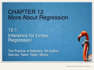
1. CHAPTER 12More About Regression 12.1 Inference for Linear Regression

2. Introduction When a scatterplot shows a linear relationship between a quantitative explanatory variable x and a quantitative response variable y, we can use the least-squares line fitted to the data to predict y for a given value of x. If the data are a random sample from a larger population, we need statistical inference to answer questions like these: • Is there really a linear relationship between x and y in the population, or could the pattern we see in the scatterplot plausibly happen just by chance? • In the population, how much will the predicted value of y change for each increase of 1 unit in x? What’s the margin of error for this estimate?

3. Sampling Distribution of b Sampling Distribution of a Slope • Choose an SRS of n observations (x, y) from a population of size N with least-squares regression line • predicted y = a + bx • Let b be the slope of the sample regression line. Then: • The mean of the sampling distribution of b is µb= b. • The standard deviation of the sampling distribution of b is • as long as the 10% Condition is satisfied. • The sampling distribution of b will be approximately normal if the values of the response variable y follow a Normal distribution for each value of the explanatory variable x (the Normal condition).

4. Conditions for Regression Inference The regression model requires that for each possible value of the explanatory variable x: • The mean value of the response variable µyfalls on the population (true) regression line µy= a + bx. • The values of the response variable y follow a Normal distribution with common standard deviation s.

5. Conditions for Regression Inference Conditions for Regression Inference Suppose we have n observations on an explanatory variable x and a response variable y. Our goal is to study or predict the behavior of y for given values of x. • Linear: The actual relationship between x and y is linear. For any fixed value of x, the mean response µy falls on the population (true) regression line µy= α + βx. • Independent: Individual observations are independent of each other. When sampling without replacement, check the 10% condition. • Normal: For any fixed value of x, the response y varies according to a Normal distribution. • Equal SD: The standard deviation of y (call it σ) is the same for all values of x. • Random: The data come from a well-designed random sample or randomized experiment.

6. How to Check Conditions for Inference Start by making a histogram or Normal probability plot of the residuals and also a residual plot. • Linear: Examine the scatterplot to check that the overall pattern is roughly linear. Look for curved patterns in the residual plot. Check to see that the residuals center on the “residual = 0” line at each x-value in the residual plot. • Independent: Look at how the data were produced. Random sampling and random assignment help ensure the independence of individual observations. If sampling is done without replacement, check the 10% condition. • Normal: Make a stemplot, histogram, or Normal probability plot of the residuals and check for clear skewness or other major departures from Normality. • Equal SD: Look at the scatter of the residuals above and below the “residual = 0” line in the residual plot. The vertical spread of the residuals should be roughly the same from the smallest to the largest x-value. • Random: See if the data were produced by random sampling or a randomized experiment.

7. Example 1 Mrs. Barrett’s class did a variation of the helicopter experiment on page 738. Students randomly assigned 14 helicopters to each of five drop heights: 152 centimeters (cm), 203 cm, 254 cm, 307 cm, and 442 cm. Teams of students released the 70 helicopters in a predetermined random order and measured the flight times in seconds. The class used Minitab to carry out a least-squares regression analysis for these data. A scatterplot and residual plot, plus a histogram and Normal probability plot of the residuals are shown below. Check whether the conditions for performing inference about the regression model are met.

8. Linear: The scatterplot shows a clear linear form. The residual plot shows a random scatter about the horizontal line. For each drop height used in the experiment, the residuals are centered on the horizontal line at 0. Independent: Because the helicopters were released in a random order and no helicopter was used twice, knowing the result of one observation should not help us predict the value of another observation. Normal: The histogram of the residuals is single-peaked and somewhat bell-shaped. In addition, the Normal probability plot is very close to linear.

9. Equal SD: The residual plot shows a similar amount of scatter about the residual = 0 line for the 152, 203, 254, and 442 cm drop heights. Flight times (and the corresponding residuals) seem to vary a little more for the helicopters that were dropped from a height of 307 cm. Random: The helicopters were randomly assigned to the five possible drop heights.

10. Constructing a Confidence Interval The confidence interval for β has the familiar form statistic ± (critical value) · (standard deviation of statistic) Because we use the statistic b as our estimate, the confidence interval is b±t* SEb We call this a t interval for the slope. t Interval for the Slope When the conditions for regression inference are met, a level C confidence interval for the slope β of the population (true) regression line is b±t* SEb In this formula, the standard error of the slope is and t* is the critical value for the t distribution with df = n - 2 having area C between -t* and t*.

11. Example 2 Earlier, we used Minitab to perform a least-squares regression analysis on the helicopter data for Mrs. Barrett’s class. Recall that the data came from dropping 70 paper helicopters from various heights and measuring the flight times. Some computer output from this regression is shown below. We checked conditions for performing inference earlier. (a) Give the standard error of the slope, SEb. Interpret this value in context. (b) Find the critical value for a 95% confidence interval for the slope of the true regression line. Then calculate the confidence interval. Show your work. (c) Interpret the interval from part (b) in context. (d) Explain the meaning of “95% confident” in context.

12. (a) We got the value of the standard error of the slope, 0.0002018, from the “SE Coef” column in the computer output. If we repeated the random assignment many times, the slope of the sample regression line would typically vary by about 0.0002 from the slope of the true regression line for predicting flight time from drop height. (b) Because the conditions are met, we can calculate a t interval for the slope β based on a t distribution with df = n − 2 = 70 − 2 = 68. Using technology: From invT(.025,68), we get t* = 1.995. The resulting 95% confidence interval is

13. (c) We are 95% confident that the interval from 0.0053218 to 0.0061270 seconds per cm captures the slope of the true regression line relating the flight time y and drop height x of paper helicopters. (d) If we repeat the experiment many, many times, and use the method in part (b) to construct a confidence interval each time, about 95% of the resulting intervals will capture the slope of the true regression line relating flight time y and drop height x of paper helicopters.

14. Performing a Significance Test for the Slope

15. Performing a Significance Test for the Slope t Test for the Slope Suppose the conditions for inference are met. To test the hypothesis H0: β = hypothesized value, compute the test statistic Find the P-value by calculating the probability of getting a t statistic this large or larger in the direction specified by the alternative hypothesis Ha. Use the t distribution with df = n - 2.

16. Example 3 Infants who cry easily may be more easily stimulated than others. This may be a sign of higher IQ. Child development researchers explored the relationship between the crying of infants 4 to 10 days old and their later IQ test scores. A snap of a rubber band on the sole of the foot caused the infants to cry. The researchers recorded the crying and measured its intensity by the number of peaks in the most active 20 seconds. They later measured the children’s IQ at age three years using the Stanford-Binet IQ test. The table below contains data from a random sample of 38 infants.  Do these data provide convincing evidence of a positive linear relationship between crying counts and IQ in the population of infants?