Download
1 / 13
210 likes | 971 Views
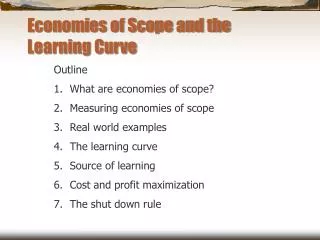
Economies of Scope and the Learning Curve. Outline What are economies of scope? Measuring economies of scope Real world examples The learning curve Source of learning Cost and profit maximization The shut down rule. Economies of Scope.

E N D
Economies of Scope and the Learning Curve • Outline • What are economies of scope? • Measuring economies of scope • Real world examples • The learning curve • Source of learning • Cost and profit maximization • The shut down rule
Economies of Scope If a single firm can jointly produce goods X and Y more cheaply that any combination of firms could produce them separately, then the production of X and Y is characterized by economies of scope This is an extension of the concept of economies of scale to the multi product case
Economies of scope can be measured by as follows: Where C(Q1,Q2) is the cost of jointly producing goods 1 and 2 in the respective quantities; C(Q1) is is the cost of producing good 1 alone, and similarly for C(Q2). Example: Let C(Q1) = $12 million; C(Q2) = $8 million; and C(Q1,Q2) = $17 million. Thus: Thus joint production of goods 1 and 2 would result in a 15 percent reduction in total costs
Economies of scope arise from “complementarities” in the production or distribution of distinct goods or services
Real world examples • Economies of scope between cable TV and high speed internet service. • Production of timber and particle board. • Corn and ethanol production • Production of beef and hides. • Power generation and distribution • Joint cargo and passenger transportation in airlines reduces excess capacity. • Global wholesale distribution of cheese, salad dressing, and cigarettes (example: Phillip-Morris-Kraft). • Computer aided design of (CAD) of aircraft components.
The Learning Curve The learning curve embodies the (inverse) relationship between average production cost and cumulative output.
Over 1,000,000,000,000,000 sold We should have this figured out by now
Sources of learning • The experience of the workforce tends to increase with cumulative output—thus workers are more familiar with the production process and have their movements/activities become routinized or a matter of habit. • There are usually several ways to do a task, and it takes time and experimentation to find the best way. • Quality control for inputs and outputs needs time to identify potential problem areas. • Input suppliers have their owning learning process
Example: Texas Instruments pushed calculator prices from about $1,000 to around $10 in the 1970s. Figure 7.6a A v e r a g e C o s t L e a r n i n g c u r v e C u m u l a t i v e O u t p u t Average cost is a decreasing function of cumulative output
Figure 7.6b A v e r a g e C o s t Learning is manifested by a downward shift of the LAC function L A C ( y e a r 1 ) I n c r e a s i n g r e t u r n s L e a r n i n g L A C ( y e a r 2 ) 1 , 0 0 0 1 , 5 0 0 R a t e o f O u t p u t ( p e r M o n t h )
Figure7.7 Costs and Profit-Maximization: The single product case D o l l a r s p e r U n i t o f O u t p u t D e m a n d ' A C M R ' ¡ P * P A C M C D e m a n d M R ¡ * Q Q Q Q ' m i n O u t p u t Green-shaded area is economic profit
Figure 7.8 Loss Minimization Means producing Some Output
Summary • If the firm shuts down production, then losses will be equal to fixed cost, or:Losses = • If the firm supplies Q* units at the price P*, then: Losses = P* Moral of the story: So long as price (average revenue) exceeds average variable cost, the loss minimizing strategy will entail producing some output.