The Learning Curve
The Learning Curve. A learning curve relates real cost to cumulative production. Given exposure to repetitive tasks: Workers learn from cumulative experience how such tasks can be performed more quickly and efficiently

The Learning Curve
E N D
Presentation Transcript
A learning curve relates real cost to cumulative production. • Given exposure to repetitive tasks: • Workers learn from cumulative experience how such tasks can be performed more quickly and efficiently • Workers include assembly line workers, plant managers, engineers, and other company officials • Machines are also affected by experience • undergo a number of technical improvements • replaced by machines embodying newer technologies
The most common form of the learning curve is Ct = C1 nta eut or in logarithms ln Ct = ln C1 + a ln nt + utwhere Ct = average real cost of production in t C1 = real unit cost in the initial production period nt = cumulative number of units produced up to but not including period t a = elasticity of unit cost with respect to cumulative volume ut = a stochastic disturbance term
Each time cumulative experience doubles, costs will decline to(100d) % of its previous level, where d = 2a or a-.50 -.33 -.25 -.16 d 0.71 0.80 0.84 0.89 fraction of previous level Ct = C1 nta eut
Better Model A better form for the learning curve which avoids biases if there are not constant returns to scale is ln Ct = 0 + 1ln nt + 2ln yt + ut nt = cumulative production (not inc. period t) yt = current production in period t
Two Studies • Two studies are based on DuPont’s production of • polyethelene • titanium dioxide. P. Ghemawat, “Building Strategy on the Experience Curve,” HBR March/April 1985 • most products fall into the ac range of -0.16 to -0.41.
Polyethelene Data YEARP UCOSTP PRODP CUMP 1960 .58 140 260 1961 .50 200 400 1962 .46 400 600 1963 .43 700 1000 1964 .39 500 1700 1965 .33 1100 2200 1966 .31 1200 3300 1967 .30 1300 4500 1968 .29 1400 5800 1969 .25 2100 7200 1970 .23 10700 9300 1971 .18 5000 20000 1972 .15 10000 25000
Polyethelene Regression The regression equation is ln_ac = 1.01 - 0.0570 ln_q - 0.221 ln_x where x is cumulative production q is current production 13 cases used 1 cases contain missing values Predictor Coef Stdev t-ratio p Constant 1.0081 0.1151 8.76 0.000 ln_q -0.05700 0.04730 -1.21 0.256 ln_x -0.22129 0.04417 -5.01 0.000 s = 0.07128 R-sq = 97.3% R-sq(adj) = 96.8% 2 -.22129 = .858
Homework p. 399 2-0.21 = .86 Exp(8.12-.21ln(800)) = 803