Download
1 / 34
390 likes | 628 Views
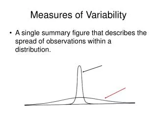
Measures of Variability. Measures of Variability. Why are measures of variability important? Why not just stick with the mean? Ratings of attractiveness (out of 10) – Mean = 5 Everyone rated you a 5 (low variability) What could we conclude about attractiveness from this?

E N D
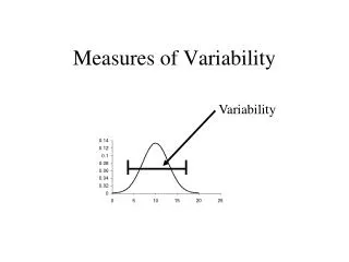
Measures of Variability • Why are measures of variability important? Why not just stick with the mean? • Ratings of attractiveness (out of 10) – Mean = 5 • Everyone rated you a 5 (low variability) • What could we conclude about attractiveness from this? • People’s ratings fell into a range from 1 – 10, that averaged a 5 (high variability) • What could we conclude about attractiveness from this?
Measures of Variability • Measures of Variability • Range • Interquartile Range • Average Deviation • Variance • Standard Deviation
Measures of Variability • Range • The difference between the highest and lowest values in a dataset • Heavily biased by outliers • Dataset #1: 5 7 11 Range = 6 Dataset #2: 5 7 11 million Range = 10,999,995
Measures of Variability • Interquartile Range • The difference between the highest and lowest values in the middle 50% of a dataset • Less biased by outliers than the Range • Based on sample with upper and lower 25% of the data “trimmed” • However this kind of trimming essentially ignores half of your data – better to trim top and bottom 1 or 5%
Measures of Variability • Average Deviation • For each score, calculate deviation from the mean, then sum all of theses scores • However, this score will always equal zero • Dataset: 19, 16, 20, 17, 20, 19, 7, 11, 10, 19, 14, 11, 6, 11, 14, 19, 20, 17, 4, 11 X = 285 285/20 = 14.25
Diff. from Mean = 0 • Mean = 0/N = 0 • www.randomizer.org
Measures of Variability • Variance • Sample Variance (s2) = (X - )2/(N-1) • Population Variance (σ2) = (X - )2/N • Note the use of squared units! • Gets rid of the positive and negative values in our “Diff. from Mean” column before that added up to 0 • However, because we’re squaring our values they will not be in the metric of our original scale • If we calculate the variance for a test out of 100, a variance of 100 is actually average variability of 10 pts. (100 = 10) about the mean of the test
(Diff. from Mean)2 = 493.75 • Variance = 493.75/(20-1) = 25.99
Measures of Variability • Standard Deviation • Sample Standard Deviation (s) = √ [(X - )2/(N-1)] • Population Standard Deviation (σ) = √ [(X - )2/N] • Note that the formula is identical to the Variance except that after everything else you take the square-root! • You can interpret the standard deviation without doing any mental math, like you did with the variance • Variance = 25.99 • Standard Deviation = √(25.99) = 5.10
Measures of Variability • Standard Deviation • Example: Bush/Cheaney – 55% Kerry/Edwards – 40% • Margin of Error = 30% Bush/Cheaney – 25% – 85% Kerry/Edwards – 10% - 70%
Computational Formula for Variability • Definitional Formula • designed more to illustrate how the formula relates to the concept it underlies • Computational Formula • identical to the definitional formula, but different in form • allows you to compute your variable with less effort • particularly useful with large datasets
Computational Formula for Variability • Definitional Formula for Variance: • s2 = (X – )2 N – 1 • Computational Formula for Variance: • s2 = • All you need to plug in here is X2 and X • Standard deviation still = √ s2, no matter how it is calculated
Computational Formula for Variability • Definitional Formula for Standard Deviation: • s = √ [(X – )2] [ N – 1 ] • Computational Formula for Standard Deviation • s = √ ( )
Computational Formula for Variability • Example: • For the following dataset, compute the variance and standard deviation. 1 2 2 3 3 3 4 5 • X = 23 • X2 = 77 • s2 = 77 – (23)2 _____8__ 8 – 1 s2 = 77 – 66.125 = 1.55 7
Measures of Variability • What do you think will happen to the standard deviation if we add a constant (say 4) to all of our scores? • What if we multiply all the scores by a constant?
Measures of Variability • Characteristics of the Standard Deviation • Adding a constant to each score will not alter the standard deviation • i.e. add 3 to all scores in a sample and your s.d. will remain unchanged • Let’s say our scores originally ranged from 1 – 10 • Add 5 to all scores, the new data ranges from 6 – 15 • In both cases the range is 9
Measures of Variability • However, multiplying or dividing each score by a constant causes the s.d. to be similarly multiplied or divided by that constant • i.e. divide each score by 2 and your s.d. will decrease from 10 to 5 • in multiplication, higher numbers increase more than lower ones do, increasing the distance between the highest and lowest score, which increases the variability • i.e. 2 x 5 = 10 – difference of 8 pts. 5 x 5 = 25 – difference of 20 pts.
Graphically Depicting Variability • Boxplot/Box-and-Whisker Plot • Median • Hinges/1st & 3rd Quartiles • H-Spread • Whisker • Outlier
Graphically Depicting Variability • Boxplot/Box-and-Whisker Plot • Median • Hinges/1st & 3rd Quartiles • H-Spread • Whisker • Outlier
Graphically Depicting Variability • Boxplot/Box-and-Whisker Plot • Median • Hinges/1st & 3rd Quartiles • H-Spread • Whisker • Outlier {
Graphically Depicting Variability • Boxplot/Box-and-Whisker Plot • Median • Hinges/1st & 3rd Quartiles • H-Spread • Whisker • Outlier
Graphically Depicting Variability • Boxplot/Box-and-Whisker Plot • Median • Hinges/1st & 3rd Quartiles • H-Spread • Whisker • Outlier
Graphically Depicting Variability • Interpreting a Boxplot/Box-and-Whisker Plot • Off-center median = Non-symmetry • Longer top whisker = Positively-skewed distribution • Longer bottom whisker = Negatively-skewed distribution
Graphically Depicting Variability • Boxplot/Box-and-Whisker Plot • Hinge/Quartile Location = (Median Location+1)/2 • Data: 1 3 3 5 8 8 9 12 13 16 17 17 18 20 21 40 • Median Location = (16+1)/2 = 8.5 • Hinge Location = (8.5+1)/2 = 4.75 (4 since we drop the fraction) • Hinges = 5 and 18
Graphically Depicting Variability • H-Spread = Upper Hinge – Lower Hinge • H-Spread = 18-5 = 13 • Whisker = H-Spread x 1.5 • Since the whisker always ends at an actual data point, if we, say calculated the whisker to end at a value of 12, but the data only has a 10 and a 15, we would end the whisker at the 10. • Whiskers = 12x1.5 = 19.5 Lower whisker from 5 to 1 Higher whisker from 18 to 21 • Outliers • Value of 40 extends beyond upper whisker
Review Questions • Central Tendency • For the following data set 1, 3, 3, 5, 5, 5, 7, 7, 9 • What is the mode? • What is the mean? • What is the median?
Review Questions • Answer: 1, 3, 3, 5, 5, 5, 7, 7, 9 • Mode = 5 • Mean = X = 45/9 = 5 • Median: • Median Location = (9 +1)/2 = 5 • Median = 5
Review Questions • Variability • For the following data set: 1 2 2 3 3 3 4 5 What is the range? What is the variance? What is the standard deviation?
Review Questions • Answer 1 2 2 3 3 3 4 5 • Range = 1 – 5 • Variance: • Mean = 2.875
Review Questions • What is the variance? • (Diff. from Mean)2 = 10.875/N – 1 = 1.55
Review Questions • What is the standard deviation? • √1.55 = 1.25