Download
1 / 67
670 likes | 1.2k Views
CENG4480_A2 Op Amps and Analog interfacing . Analog interfacing techniques. Computer interfacing Introduction. To learn how to connect the computer to various physical devices. Some diagrams of this manuscript are taken from the following references:

E N D
CENG4480_A2 Op Amps and Analog interfacing Analog interfacing techniques op-amps (v.1a)
Computer interfacing Introduction • To learn how to connect the computer to various physical devices. • Some diagrams of this manuscript are taken from the following references: • [1] S.E. Derenzo, Interfacing -- A laboratory approach using the microcomputer for instrumentation, data analysis and control prentice hall. • [2] D.A. Protopapas, Microcomputer hardware design, Prentice hall • [3] G C Loveday, Designing electronic hardware, Addison Wesley op-amps (v.1a)
Topics include: • Overall interfacing schemes • Analog interface circuits, active filters • Analog/digital conversions • sensors, controllers • Control techniques • Advanced examples op-amps (v.1a)
Overall view: a typical data acquisition and control system Timer e.g. 8253 Digital control circuit Sensor Computer filter Sample & Hold A/D Op-amp Mechanical device Power circuit D/A op-amps (v.1a)
Analog interface example1 Audio recording systems • Audio recording systems • Audio signal is 20~20KHz • Sampling at 40KHz, 16-bit is Hi-fi • Stereo ADC require to sample at 80KHz. • Calculate storage requirement for one hour? • Audio recording standards • Audio CD • Mini-disk MD • MP3 op-amps (v.1a)
Analog interface example2 Surround sound audio systems • A common two channels audio CD • Calculate storage size for one hour of recording of a CD. 44.1KHz*2bytes*60sec*60min*2 channels=633.6Mbytes • Calculate the play time of a CD. 700M/(2bytes*44.1KHz*2channels*60sec)=61.4 minutes • 6 Channels: Front R/L,Rear R/L, Middle, Sub woofer • 44.1KHz, • Calculate the sampling frequency. op-amps (v.1a)
Analog interface example3Play stations and Wii • Play station 3, Analog hand held controller (http://ryangenno.tripod.com/images/PlayStation3-system.gif) • Wii, http://www.onlinekosten.de/news/bilder/wii_controller.jpg • Driving wheel http://www.bizrate.com/gamecontrollers/logitech-driving-force-driving-force-wheel--pid11297651/ op-amps (v.1a)
Operational Amplifier choices (op amp) • Why use op amp? • What kinds of inputs/outputs do you want? • What frequency responses do you want? op-amps (v.1a)
Source load requirements: DC ( static or slow changing, without decoupling capacitors) AC( for fast changing signal, use decoupling capacitors) Input range, biased – absolute min, max voltage Output range, biased – absolute min, max voltage Frequency: range, allowed attenuation in dB Noise tolerance Power – output current/output impedance. DC-direct current amplifier AC-alternating current amplifier Factors for choosing an amplifier DC Source Op- amp Load AC Source Op- amp Load op-amps (v.1a)
Discussions: what kind of amplifiers should we use? It is an art. • Condenser microphone(+/-10mV) • Audio amplifier from MP3 player to speaker • Ultrasonic sensors (+/-1mV) to ADC (analog to digital converter) (0-5V) • Accelerometers (+/-5V), or (+/-500mV) • Temperature sensors to ADC (010mv) • Moving coil microphone with 50Hz noise (+/-0.5mV) op-amps (v.1a)
Suggestions • Condenser microphone(+/-100mV): AC, bandwidth=audio range(20-20KHz, voltage gain ~=100,low power. • Moving coil microphone with 50Hz noise (+/-0.5mV): AC, bandwidth=audio range, voltage gain ~=2000,low power. • Audio amplifier from MP3 player to speaker: AC, high power, voltage gain ~=5, power gain~=100, bandwidth=audio range • Ultrasonic sensors (+/-1mV) to ADC (0-5V): DC-shift needed, voltage gain~=5000. bandwidth=tuned narrow band • Accelerometers (+/-500mV): DC-shift needed, voltage gain ~=10, • Temperature sensors to ADC (010mv): DC, voltage gain~=100. op-amps (v.1a)
Operational amplifiers (op-amps) • ideal op-amps • inverting amplifier • non-inverting amplifier • voltage follower • current-to-voltage amplifier • summing amplifier • full-wave rectifier • instrumental amplifier op-amps (v.1a)
General concept about OP amps • Controllable gain • For DC or AC amplifier • Not too high frequency responses op-amps (v.1a)
Ideal Vs. realistic op-amp • Ideal Realistic Rin • A= infinite 105->108 • Zin= infinite 106(bipolar input) 1012(FET input)output offset exists 2 3 _ V- 6 V0=A(V+-V-) LM741 + V+ + op-amps (v.1a)
Inverting amplifier • Gain(G) = -R2/R1 • For min. output offset, set R3 = R1 // R2 • Rin=R1 Virtual-ground,V2 R2 _ V1 R1 V0 A + R3 + op-amps (v.1a)
Non-inverting amplifier • Gain(G) 1 + (R2/R1) • For min. offset output , set R1//R2=Rsource • High input resistance V1 + A V0 _ R2 V2 R1 op-amps (v.1a)
Differential amplifier • V0=(R2/R1)(V2-V1) • Minimum output offset R1 //R2 =R3 //R4 R2 R1 _ V1 V0 A V2 + R3 R4 op-amps (v.1a)
Exercise 1 • A temperature sensor has an offset of 100mV (produces an output of 100mV at 0 °C-degrees Celsius), and the gradient is 10 mV per °C. The temperature to be measured is ranging from 0 to 50 °C. • The required ADC input range is 0 to 9Volts. • Given that the power supply is +/-9V, design a differential amplifier for this application. op-amps (v.1a)
Voltage follower (Unit voltage gain, high current gain, high input impedance) • Gain=1, • Rin=high • For minimum output offset R=Rsource V1 + V0=V1 A _ R op-amps (v.1a)
Current to voltage converter: application to photo detector – no loading effect for the light detector • V0=I R • I should not be too large otherwise offset voltage will be too high. Photodiode Light detector R I _ V0 A + See http://hyperphysics.phy-astr.gsu.edu/hbase/electronic/photdet.html#c1 op-amps (v.1a)
Summing amplifier • V0 = -{(V1/R1)+(V2/R2)+(V3/R3)}R I1 R V1 R1 _ V2 R2 V0 I1+I2+I3 + V3 R3 op-amps (v.1a)
Op-amp characteristics • Input and output offset voltages • It is affected by power supply variations, temperature, and unequal resistance paths. • Some op-amps have offset setting inputs. • Unequal resistance paths and bias currents on inverting and non-inverting inputs • Temperature variations -- read data sheet for operating temperatures op-amps (v.1a)
Op-amp dynamic response • Slew rate -- the maximum rate of output change (V/us) for a large input step change. • A741 slew rate=0.5V/ s. Fast slew rate is important in video circuits , fast data acquisition etc. • Gain bandwidth product • higher gain --> lower frequency response • lower gain --> higher frequency response op-amps (v.1a)
Common mode gain • If the two inputs (V+,V-) are connected together and is given Vc, output is found to be Vo. • ideal differential amplifier only amplifies the voltage difference between its two inputs, so Vo should be 0. • But in practice it is not. • This deficiency can be measured by the Common mode gain=Vo/Vc. op-amps (v.1a)
Diagram of gain bandwidth product, from [1] op-amps (v.1a)
Instrumental amplifierTo make a better DC amplifier from op-amps Applications: DSO input amplifiers, amplifiers in medical measurement systems op-amps (v.1a) Diagram of instrumental amplifier, from [1]
Instrumental amplifier • It has all the advantages of an amplifier. • Gain(G)=V0/(V+-V-) • =(R4/R3)[1+(2R2/R1)] (typically 10 to 1000) • Even V+=V-= Vc, there is a slight output because of the Common Mode Gain=Gc=V0/Vc • Therefore, V0= G(V+-V-)+GcVc • To measure this imperfection, Common Mode rejection ratio (CMRR)=G/Gc (typically 103 to 107, or 60 to 140 dB)is used , the bigger the better. op-amps (v.1a)
Comparing amplifiers, from [1] • Op Inv. Noninv. Diff. Instu. • Amp Amp Amp Amp Amp • High Rin Yes No Yes No Yes • Diff’tial Yes No No Yes Yes • input • Defined No Yes Yes Yes Yes • gain op-amps (v.1a)
Operational amplifier selection techniques and keywords • National semiconductor is the main manufacturer: See http://www.national.com/appinfo/milaero/analog/highp.html • General Purpose: LM741* • High Slew Rate:50V/ ms --> 2000V/ ms (how fast the output can be changed) • Follower (high speed):50MHz • Low Supply Current: 1.5mA --> 20 µA/Amp • Low offset voltage: 100 µV • Low Noise • Low Input Bias Current: 50pA -->10pA • High Power : 0.2A --> 2A • Low Drift: 2.5 mV/ _C --> 1.0 mV/ _C • Dual/Quad • High Power Bandwidth High Power Bandwidth : 300KHz - 230Mhz op-amps (v.1a)
Practical op-amp usage examples • Example 1: Working with one power supply • Example 2: Active filters • Example 3: Sample and hold • Example 4: Example 4: Voltage Comparator and schmit trigger • Example 5: Power amplifier op-amps (v.1a)
Example 1: Single power supply for op-amps • Small systems usually have 1 power supply • Output V0 is biased at E/2 rather than 0. • E.g. Inverting amplifier. GainR2/R1 Vo R2 E/2 E _ E/2 V1 R1 V+ V- A Vo + R3 + 0-Volt 0-Volt R=20K R=20K E Volts Power supply E/2 op-amps (v.1a)
Typical AC amplifier design Condenser microphone amplifier circuit, and the diagram showing the output swing around the biased 2.5V. The capacitors isolate the stages. Condenser MIC output impedance is 75 Ohms What is the input impedance of the amplifier? op-amps (v.1a)
Example 2: Active filters (analog and using op-amps) • Applications: accept or reject certain signals with specific frequencies. High-pass, low-pass, band-pass etc. E.g. • reject noise • extract signal after demodulation • reject unwanted side effect signals op-amps (v.1a)
Types • 2-1: Low pass • 2-2: High pass • 2-3: Band stop (notch): e.g. noise removal • 2-4: Band pass op-amps (v.1a)
definition of power gain in decibel (dB) • Output power is P2, input power is P1 • Power Gain in dB=10 log10 (P1/P2) • Or • Output voltage is V2, input voltage is V1 • Assume load R is the same, power=V2/R • Power Gain in dB=10 log10 (V12/ V22) • Power Gain in dB=20 log10 (V1/ V2) op-amps (v.1a)
Important terms for filters: Formulas are not important, remember the frequency-gain curve and concepts • Pass band-- range of frequency that are passed unfiltered • Stop band -- range of frequency that are rejected. • Corner frequency -- where amplitude dropped by 2-1/2=0.707= -3dB • I.e. in dB: 20log(0.707) = -3dB • Settling time -- time required to rise within 10% of the final value after a step input. op-amps (v.1a)
2-1 Low pass • Only low frequency signal can pass • one-pole: attenuates slower 20dB/decade • two-pole: attenuates faster 40dB/decade • Applications: • remove high freq. Noise, • remove high freq. before sampling to avoid aliasing noise op-amps (v.1a)
Diagram for low-passone pole filter, from [1]for simplicity make R2/R1=1, gain 20 dB/decade drop • -R2/R1 • |G| = ------------------- • {1+(f/fc)2}1/2 3dB fc Freq. op-amps (v.1a)
Formula, also op-amps (v.1a)
2-1aLow pass, one pole filter formulas for simplicity make R2/R1=1 • -R2/R1 • |G| = ------------------- • {1+(f/fc)2}1/2 • Corner frequency= fc=1/(2R2C) • The gain drops 6dB/octave or 20 dB/decade op-amps (v.1a)
Diagram for Low-passtwo-pole filter, from [1] for simplicity make R3/(R2+R1)=1 40 dB/decade drop gain 6dB • - R3/(R2+R1) • |G|= ------------------ • 1+(f/fc)2 fc Freq. op-amps (v.1a)
2-1bLow-passtwo-pole filter formulas for simplicity make R3/(R2+R1)= 1 • - R3/(R2+R1) • |G|= ------------------ • 1+(f/fc)2 • Corner frequency=fc • fc=(R1//R2)/2C1 =(2 R3C2)-1 when gain G drops at -6dB. • G is dropping at 40dB/decade op-amps (v.1a)
Matlab, lp42.m • %lp42.m, ceg3480 matlab demo %low pass filter-one pole • clear • f=[0:100:2000] • N=length(f) • fc=1000 • for i=1:N • % -----gain1 , low pass one pole , for simplifcity make (R2/R1)=1 • gv1(i)=-1/sqrt(1+(f(i)/fc)^2); • %db=10*log_base10(power1/power2); or dB=20*log_base10(voltage1/voltage2; • gain1_db(i)=20*log10(abs(gv1(i))); • % -----gain2 , low pass two pole , for simplifcity make {R3/(R1+R2)}=1 • gv2(i)=-1/(1+(f(i)/fc)^2); • %db=10*log_base10(power1/power2); or dB=20*log_base10(voltage1/voltage2; • gain2_db(i)=20*log10(abs(gv2(i))); • end • % %======================================================== • figure(1) • clf • limit_y=min(gain2_db) • semilogx(f,gain1_db,'g-.') • hold on • semilogx(f,gain2_db,'b--') • %------------------------ • semilogx([fc,fc],[0,limit_y],'k-.') • legend('one pole','two pole','fc=1000',4); • %------------------------------------------------------- • semilogx(f,ones(N)*-3,'r') • text(f(N),-3,'- 3d B line') • %------------------------ • semilogx(f,ones(N)*-6,'r') • text(f(N),-6,'- 6d B line') • ylabel('low pass filter gain in d B') • xlabel('freq Hz f in log scale') op-amps (v.1a)
Plotting the comparison of the low pass filters (one-pole, two-pole) op-amps (v.1a)
2-2High pass • Only high frequency signal can pass • one-pole: attenuates slower 20dB/decade • two-pole: attenuates faster 40dB/decade • Applications: • Remove low freq. Noise (50Hz main) • Remove DC offset drift. op-amps (v.1a)
2-2aDiagram for high-passone-pole filter, from [1]For simplicity make R1=R2 20 dB/decade drop • (f/fc) • |G|=------------------- • {1+(f/fc)2}1/2 • fc=1/{2 (R1C)} gain 3dB fc Freq. high freq. Cutoff unintentionally Created by Op-amp op-amps (v.1a)
High-passone-pole filter formulas • (f/fc) • |G|=------------------- • {1+(f/fc)2}1/2 • Corner frequency= fc=1/{2 (R1C)} • At low f , |G|=f/fc; at high f , |G|=R2/R11 • Since op-amp has a certain gain-bandwidth, so at high frequency the gain drops. So all op-amp high-pass filters are actually band-pass. op-amps (v.1a)
Matlab hp52.m • %hp52.m ceg3480 matlab demo %high pass filter-one pole • clear • f=[500:100:100000] • N=length(f) • fc=1000 • for i=1:N • % -------------------gain3 , high pass ,one pole • gv3(i)=-(f(i)/fc)/sqrt(1+(f(i)/fc)^2); • %db=10*log_base10(power1/power2); or dB=20*log_base10(voltage1/voltage2; • gain3_db(i)=20*log10(abs(gv3(i))); • end • % %======================================================== • figure(1) • clf • limit_y=min(gain3_db) • semilogx(f,gain3_db,'k-.') • hold on • %------------------------ • semilogx([fc,fc],[0,limit_y],'g-.') • legend('one pole','fc=1000',4); • %------------------------------------------------------- • semilogx(f,ones(N)*-3,'r') • text(f(N),-3,'- 3d B line') • ylabel('high pass filter gain in d B') • xlabel('f freq in log scale') op-amps (v.1a)
high pass one pole filter op-amps (v.1a)
2-3Band stop (notch) filter • Suppresses a narrow frequency band of signal op-amps (v.1a)