Download

1 / 71
720 likes | 841 Views
This presentation explores the Random Knapsack problem and its resolution in expected polynomial time using a dominating set approach. Guided by Professor 呂學一, team members 陳姿樺, 何明彥, and 余宗恩 delve into analyzing the algorithm's effectiveness under uniform distributions, long-tailed distributions, and general cases. The discussion covers key concepts like domination, the Nemhauser/Ullmann algorithm, and applications of the theory, providing insights into expected performance and a lower bound for the expected number of dominating sets.

E N D
Team members • R91921028 陳姿樺 • R92921084 何明彥 • R92921083 余宗恩
Outline • Introduction…………………………姿樺 • The uniform distribution…………姿樺 • Long-tailed distributions • Analysis……………………………………姿樺 • Applications………………………………明彥 • Lower bound…………………………明彥 • General distributions………………宗恩
Introduction • Speaker : R91921028 陳姿樺
Today • Random Knapsack in Expected Polynomial Time
The problem • Input : • Given n items with positive weights w1, . . . ,wn • and profits p1, . . . , pn • and a knapsack capacity c, • Output : • find a subset S [n] :={1,2, . . . ,n} such that ∑iS wic and ∑iS pi is maximized.
Domination concept • Two subset: • A subset S [n] with weight w(S)=∑iSwi and profit p(S) = ∑iSpi • Another subset T [n] with weight w(T)=∑iT wi and profit p(T) = ∑iTpi • We say S dominates T if w(S) w(T) and p(S) p(T).
Assume • For simplicity assume that no two subsets have the same profit.
Example • n=3 • S={1,3}; w(S)=3; p(S)=1.4 • T={1,2}; w(T)=5; p(T)=0.8 • S dominates T
observation • No subset dominated by another subset can be an optimal solution to the knapsack problem, regardless of the specified knapsack capacity. • It suffices to consider those sets that are not dominated by any other set, the so-called dominating sets.
observation • In the dominating sets, the solutions that cannot be improved in weight and profit simultaneously by other solutions. • Why? • By domination concept
The Nemhauser/Ullmann algorithm • For i [n], let S(i) be the sequence of dominating subsets over the items 1,...,i. • The sets in S(i) are assumed to be listed in increasing order of their weights.
The Nemhauser/Ullmann algorithm • Given S(i), S(i+1) can be computed as follows: • duplicate all subsets in S(i) and then add item i+1 to each of the duplicated sets. • Removing the sets dominated by any other set. • The result is the ordered sequence S(i+1) of dominating sets over the items 1, . . . , i+1.
Example • n=3
Naïve algorithm • List total state and find dominating set • 21=0,1; • S(1)={0,1} • 22=0,1,2,12; • S(2)={0,1,12} • 23=0,1,2,3,12,13,23,123; • S(3)={0,3,13,123}
Nemhauser/Ullmann algo. • S(1)={0,1} • Find S(2) • From {0,1,2,12} to find dominating set • S(2)={0,1,12} • Find S(3) • From {0,1,12,3,13,123} to find • S(3)={0,3,13,123} • The same as naïve algorithm
Something • Let us assume that add and compare numbers in constant time. • Then the sequence S(i+1) can be calculated from the sequence S(i) in time linear. • The optimal knapsack filling is described by one of the subsets in the list S(n) • Generating S(n) basically solves the knapsack problem.
Lemma • For every i[n], let q(i) denote an upper bound on the (expected) number of dominating sets over the items in 1,...,i, and assume q(i+1) q(i). The Nemhauser/Ullmann algorithm computes an optimal knapsack filling in (expected) time
By the lemma • We can only think the number of dominating sets, i.e., q(n) • Goal: counting E[q]
THE UNIFORM DISTRIBUTION • Assumption: • Profits are assumed to be chosen uniformly at random from [0,1] and, • In all of our analyses, weights are chosen by an adversary.
Definition • Let m=2n and let S1,...,Sm denote the sequence of all subsets of [n] listed in non-decreasing order of their weights. • Let the profit of subset Su be Pu=ΣiSu pi. • For any 2 u m, define Δu=maxv[u]Pv - maxv[u-1] Pv 0.
Observation • Observe that S1 is always a dominating set. • For all u 2, Su is dominating if and only if Δu > 0.
Example • n=3 • Su
Example • Δ2=P2 - P1 =0.9 • Δ3=P2 - P2 =0 • Δ4=P2 - P2 =0 • Δ5=P5 - P2 =0.5 • Δ6=P5 - P5 =0 • Δ7=P5 - P5 =0 • Δ8=P8 - P5 =0.3 • Dominating sets: S1, S2, S5, S8,
Lemma • For every u {2,...,m},
Theorem • Suppose the weights are arbitrary positive numbers and profits are chosen according to the uniform distribution over [0,1]. Let q denote the number of dominating sets over all n items. Then E[q] = O(n3).
Proof theorem • Pm=ΣiSmpi=Σi[n]pi and P1=ΣiS1pi=0 • E[Pm]=n/2 because each individual item has profit 1/2 on expectation. P1=0 By lemma
Proof theorem • Consequently,
Proof Lemma(1) • For every u {2,...,m},
Proof Lemma(2) • Find a easy way • The goal is change to
Definition • For every v[u-1], define Xv=Su\Sv and Yv=Sv\Su. • Lv=∑iXvpi • Define two set • Clearly, AB
Definition • For ε[0,1], we define • Obviously, B=B0 and, in general, Bε can be obtained by shrinking B in each dimension by a factor of 1-ε. • As the number of dimensions is n-k, it holds
Help1 • Lv1/4n • Proof:
Help1 • we assume pj 1/4n, for every j[k]. • Lv=∑iXvpi, Under our assumption, Lv 1/4n, for every v[u-1], • Why? • because each set Xv contains at least one element of size at least 1/4n .
Help2 • Observe that Lv(1-1/4n ) Lv-1/16n2 because Lv1/4n. Thus setting ε=1/4n implies Bε A.
Proof new Lemma By definition By help2
Long-tailed vs. short-tailed • if the tail function of a distribution can be lower-bounded by the tail function of the exponential function, then we say the distribution has a “long tail”, and if the tail function can be upper-bounded by the exponential tail function, then we talk about “short tails”.
Definition • Given any continuous probability distribution with density function f:R0→R0, the tail function T:R0→[0,1] is defined by T(t)=∫t∞f(x)dx. • We define the slope of T at xR0 to be the first derivative of the function -ln(T(·)) at x, i.e., slopeT(x)=-[ln(T(x))]’.
Long-tailed definition • The tail of a continuous probability distribution is defined to be long if there exists α>0 such that slopeT(x) α, for every xR 0.
Theorem • For i[n], let profit pi be a random variable with tail function Ti:R 0→[0,1]. Define µi = E[pi] and let αi be an appropriate positive real number satisfying slopeTi(x)αi for every x0, i[n]. Let α=maxi[n]αi and µ=maxi [n]µi. Finally, let q denote the number of dominating sets over the elements in [n]. • Then
Proof theorem • µi = E[pi], so E[Pm]=∑i[n]µi. • Help3: • Proof of theorem
Help3 • Help3 can be proved by the former lemma
Part II • Speaker : R92921084 何明彥
Application(1/2) • by theorem: if profits are chosen according to the exponential distribution ,then
Application(2/2) • The exponential and other long tailed distribution: • We can generalize the upper bound towards all continuous distributions with finite mean.
Goal • a lower bound for the number of dominating set for continuous distributions with non-increasing density function.
Theorem(1/4) • draw profitrandomly according to a continuous probability distribution with non-increasing density function: • then a vector of weight w1,…,wn • Therefore,
Theorem(2/4) • : the weight for i-th item • : the profit • For every jn • : the dominating set for item 1,…j-1