Understanding Discrete Random Variables: Expectations, Sums, and Binomial Models
This article delves into discrete random variables and essential concepts like probability mass functions (p.m.f.), expected values, and the linearity of expectation. We explore practical examples, including coin flips and dice rolls, to illustrate these principles. The article further discusses the binomial random variable, its properties, and variance calculation. By the end, readers should grasp how to compute expectations and variances in various scenarios, including drawing balls from an urn and investment choices with uncertainty.


Understanding Discrete Random Variables: Expectations, Sums, and Binomial Models
E N D
Presentation Transcript
Review A discrete random variableX assigns a discrete value to every outcome in the sample space. E[N] • Probability mass function of X: p(x) = P(X = x) Expected value of X: E[X] = ∑xx p(x). N: number of headsin two coin flips
One die Example from last time F = face value of fair 6-sided die E[F] = 1 + 2 + 3 + 4 + 5 + 6 = 3.5 1 1 1 1 1 1 6 6 6 6 6 6
Two dice S = sum of face values of two fair 6-sided dice 1 2 5 3 5 4 4 3 2 1 6 36 36 36 36 36 36 36 36 36 36 36 Solution 1 We calculate the p.m.f. of S: 2 3 4 5 6 7 8 9 10 11 12 s pS(s) 1 2 1 36 36 36 E[S] = 2 + 3 + … + 12 = 7
Two dice again S = sum of face values of two fair 6-sided dice F1 F2 S = F1+ F2 F1 = outcome of first die F2 = outcome of second die
Sum of random variables Let X, Y be two random variables. Xassigns value X(w) to outcome w Y assigns value Y(w) to outcome w X + Yis the random variable that assigns value X(w)+ Y(w) to outcome w.
Sum of random variables S = F1+ F2 F1 F2 2 1 1 11 3 1 2 12 … … 3 2 1 21 … … 12 6 6 66
Linearity of expectation For every two random variables X and Y E[X + Y] = E[X] + E[Y]
Two dice again S = sum of face values of two fair 6-sided dice F1 F2 Solution 2 S = F1+ F2 E[S] = E[F1] + E[F2] = 3.5 + 3.5 = 7
Balls We draw 3 balls without replacement from this urn: 0 -1 1 0 1 -1 1 -1 -1 What is the expected sum of values on the 3 balls?
Balls 0 -1 1 0 S = B1 + B2 + B3 1 -1 1 3 2 4 -1 -1 where Bi is the value of i-th ball. 9 9 9 E[S] = E[B1] + E[B2] + E[B3] -1 0 1 x p.m.f of B1: p(x) E[B1] = -1 (4/9) + 0 (2/9) + 1 (3/9) = -1/9 same for B2, B3 E[S] = 3 (-1/9) = -1/3.
Three dice N = number of s. Find E[N]. I3 I2 I1 Solution 1 if face value of kth die equals Ik= 0 if not N = I1 + I2 + I3 = 1/2 E[N] = E[I1] + E[I2] + E[I3] = 3 (1/6) E[I1] = 1 (1/6) + 0(5/6) = 1/6 E[I2], E[I3] = 1/6
Problem for you to solve Five balls are chosen without replacement from an urn with 8 blue balls and 10 red balls. (a) What is the expected number of blue balls that are chosen? (b) What if the balls are chosen with replacement?
The indicator (Bernoulli) random variable Perform a trial that succeeds with probability p and fails with probability 1 – p. p(x) x 0 1 p(x) 1 – p p p= 0.5 If X is Bernoulli(p) then p(x) E[X] = p p= 0.4
The binomial random variable Binomial(n, p): Perform n independent trials,each of which succeeds with probability p. X= number of successes Examples Toss n coins. “number of heads” is Binomial(n, ½). Toss n dice. “Number of s” is Binomial(n, 1/6).
A less obvious example Toss n coins. Let C be the number of consecutive changes (HT or TH). w C(w) Examples: • HHHHHHH • 0 • THHHHHT • 2 • HTHHHHT • 3 Then C is Binomial(n – 1, ½).
A non-example Draw a 10 card hand from a 52-card deck. Let N = number of aces among the drawn cards Is N a Binomial(10, 1/13)random variable? No! • Trial outcomes are notindependent.
Properties of binomial random variables If X is Binomial(n, p), its p.m.f. is p(k) = P(X = k) = C(n, k) pk (1 - p)n-k We can write X = I1 + … + In, where Ii is an indicator random variable for the success of the i-th trial E[X] = E[I1] + … + E[In] = p + … + p = np. E[X] = np
Probability mass function Binomial(10, 0.5) Binomial(50, 0.5) Binomial(10, 0.3) Binomial(50, 0.3)
Functions of random variables p.m.f. of X: p.m.f. of X - 1: x 0 12 y -1 0 1 p(x) p(y) 1/3 1/3 1/3 1/3 1/3 1/3 p.m.f. of (X – 1)2: y 0 1 p(y) 1/3 2/3 If X is a random variable, then Y = f(X) is a random variable with p.m.f. pY(y) = ∑x: f(x) = ypX(x).
Investments You have two investment choices: A: put $25 in one stock B: put $½ in each of 50 unrelated stocks Which do you prefer?
Investments Probability model doubles in value with probability ½ Each stock loses all value with probability ½ Different stocks perform independently
Investments A: put $50 in one stock B: put $½ in each of 50 stocks NA = amount on choice A NB = amount on choice B 50 × Bernoulli(½) Binomial(50, ½) E[NB] E[NA]
Variance and standard deviation Let m = E[X] be the expected value of X. The variance of X is the quantity Var[X] = E[(X – m)2] The standard deviation of X is s = √Var[X] It measures how close X and m are typically.
Calculating variance m = E[NA] x 0 50 p(x) ½ ½ m –s m +s p.m.f of NA y 252 Var[NA] = E[(NA – m)2] = 252 q(y) 1 s= std. dev. of NA = 25 p.m.f of (NA– m)2
Another formula for variance for constant c, E[cX] = cE[X] Var[X] = E[(X – m)2] for constant c, E[c] = c = E[X2 – 2mX +m2] = E[X2] + E[–2mX]+E[m2] = E[X2] – 2m E[X]+m2 = E[X2] – 2mm+ m2 = E[X2] – m2 Var[X] = E[X2] – E[X]2
Variance of binomial random variable Suppose X is Binomial(n, p). 1, if trial isucceeds Then X = I1 + … + In, where Ii = 0,if trial i fails • m = E[X] = np = np + n(n-1) p2– (np)2 • Var[X] = E[X2] – m2 = E[X2] – (np)2 • E[X2] = E[(I1 + … + In)2] = E[I12+ … + In2 + I1I2 + I1I3 + … + InIn-1] = E[I12] + … + E[In2]+ E[I1I2] + … + E[InIn-1] • = n p • = n(n-1) p2 • E[Ii2] = E[Ii] = p • E[Ii Ij] = P(Ii = 1 andIj= 1) • = P(Ii = 1) P(Ij= 1) = p2
Variance of binomial random variable Suppose X is Binomial(n, p). m = E[X] = np • Var[X] = np + n(n-1) p2 – (np)2 • = np – np2= np(1-p) Var[X] = np(1-p) The standard deviation of X is s= √np(1-p).
Investments A: put $50 in one stock B: put $½ in each of 50 stocks NA = amount on choice A NB = amount on choice B 50 × Bernoulli(½) Binomial(50, ½) m m m –s m +s s= 25 s= √50½ ½ = 3.536…
Average household size In 2011 the average household in Hong Kong had 2.9 people. Take a random person. What is the average number of people in his/her household? B: 2.9 C: > 2.9 A: < 2.9
Average household size averagehousehold size 3 3 average size of randomperson’s household 4⅓ 3
Average household size What is the average household size? household size 1 2 3 4 5 more % of households 16.6 25.6 24.4 21.2 8.7 3.5 From Hong Kong Annual Digest of Statistics, 2012 Probability model The sample space are the households of Hong Kong Equally likely outcomes X = number of people in the household E[X] ≈ 1×.166 + 2×.256 + 3×.244 + 4×.214 + 5×.087 + 6×.035 = 2.91
Average household size Take a random person. What is the average number of people in his/her household? Probability model The sample space are the people of Hong Kong Equally likely outcomes Y = number of people in household Let’s find the p.m.f. pY(y)=P(Y = y)
Average household size household size 1 2 3 4 5 more % of households 16.6 25.6 24.4 21.2 8.7 3.5 N = number of people in Hong Kong H = number of households in Hong Kong ≈ 1×.166H + 2×.256H + 3×.244H + 4×.214H + 5×.087H + 6×.035H • N pY(1) =P(Y = 1) = 1×.166H/N pY(2) =P(Y = 2) = 2×.256H/N pY(y) = P(Y = y) = y×pX(y)/E[X] = y×P(X= y) H/N
Average household size X = number of people in a random household Y = number of people in household of a random person y pX(y) ∑yy2pX(y) pY(y) = E[Y] = ∑yy pY(y) = • E[X] • E[X] household size 1 2 3 4 5 more % of households 16.6 25.6 24.4 21.2 8.7 3.5 12×.166 + 22×.256 + 32×.244 + 42×.214 + 52×.087 + 62×.035 ≈ 3.521 E[Y] ≈ • 2.91
Preview X = number of people in a random household Y = number of people in household of a random person • E[X2] E[Y] = • E[X] Because Var[X] ≥ 0, E[X2] ≥ (E[X])2 So E[Y]≥ E[X]. The two are equal only if all households have the same size.
This little mobius strip of a phenomenon is called the “generalized friendship paradox,” and at first glance it makes no sense. Everyone’s friends can’t be richer and more popular — that would just escalate until everyone’s a socialite billionaire. • The whole thing turns on averages, though. Most people have small numbers of friends and, apparently, moderate levels of wealth and happiness. A few people have buckets of friends and money and are (as a result?) wildly happy. When you take the two groups together, the really obnoxiously lucky people skew the numbers for the rest of us. Here’s how MIT’s Technology Review explains the math: • The paradox arises because numbers of friends people have are distributed in a way that follows a power law rather than an ordinary linear relationship. So most people have a few friends while a small number of people have lots of friends. • It’s this second small group that causes the paradox. People with lots of friends are more likely to number among your friends in the first place. And when they do, they significantly raise the average number of friends that your friends have. That’s the reason that, on average, your friends have more friends than you do. • And this rule doesn’t just apply to friendship — other studies have shown that your Twitter followers have more followers than you, and your sexual partners have more partners than you’ve had. This latest study, by Young-Ho Eom at the University of Toulouse and Hang-Hyun Jo at Aalto University in Finland, centered on citations and coauthors in scientific journals. Essentially, the “generalized friendship paradox” applies to all interpersonal networks, regardless of whether they’re set in real life or online. • So while it’s tempting to blame social media for what the New York Times last month called “the agony of Instagram” — that peculiar mix of jealousy and insecurity that accompanies any glimpse into other people’s glamorously Hudson-ed lives — the evidence suggests that Instagram actually has little to do with it. Whenever we interact with other people, we glimpse lives far more glamorous than our own. • That’s not exactly a comforting thought, but it should assuage your FOMO next time you scroll through your Facebook feed.
Zoe Bob Sam X = number of friends Alice Y = number of friends of a friend Jessica Mark Eve In your homework you will show that E[Y] ≥ E[X] in any social network
Apples About 10% of the apples on your farm are rotten. You sell 10 apples. How many are rotten? Probability model Number of rotten apples you sold isBinomial(n = 10, p = 1/10). E[N] = np = 1
Apples You improve productivity; now only 5% apples rot. You can now sell 20 apples and only one will be rotten on average. N is now Binomial(20, 1/20).
.387 Binomial(10, 1/10) .349 .194 10-10 .001 .377 .354 Binomial(20, 1/20) .189 .002 10-8 10-26 .367 .367 .183 10-19 .003 10-7
The Poisson random variable A Poisson(m) random variable has this p.m.f.: p(k) = e-mmk/k! k = 0, 1, 2, 3, … Poisson random variables do not occur “naturally” in the sample spaces we have seen. They approximateBinomial(n, p) random variables when m = np is fixed and n is large (so p is small) pPoisson(m)(k) = limn → ∞pBinomial(n, m/n)(k)
Raindrops Rain is falling on your head at an average speed of 2.8 drops/second. 0 1 Divide the second evenly in n intervals of length 1/n. Let Ei be the event “raindrop hits during interval i.” Assuming E1, …, En are independent, the number of drops in the second Nis a Binomial(n, p)r.v. Since E[N] = 2.8, and E[N] = np, pmust equal 2.8/n.
Raindrops 0 1 Number of drops N is Binomial(n, 2.8/n) As n gets larger, the number of drops within the second “approaches” a Poisson(2.8) random variable:
Expectation and variance of Poisson If X is Binomial(n, p) then E[X] = np Var[X] = np(1-p) When p = m/n, we get E[X] = m Var[X] = m(1-m/n) As n→ ∞,E[X]→ mandVar[X] →m. This suggests • When X is Poisson(m), E[X]= mandVar[X] = m.
Problem for you to solve Rain falls on you at an average rate of 3 drops/sec. When 100 drops hit you, your hair gets wet. You walk for 30 sec from MTR to bus stop. What is the probability your hair got wet?
Problem for you to solve Solution On average, 90 drops fall in 30 seconds. So we model the number of drops N you receive as a Poisson(90) random variable. Using the online Poisson calculator at or the poissonpmf(n, L) function in 14L07.py we get P(N > 100) = 1 - ∑i= 0 P(N = i) ≈ 13.49% 99