Download

1 / 34
340 likes | 452 Views
This article explores the concept of discrete random variables and their impact on the probability mass function (p.m.f.). A discrete random variable assigns distinct values to outcomes in a sample space, illustrated through examples such as coin tosses and ball draws. The p.m.f. is defined, demonstrating how to calculate probabilities for given outcomes, and how to represent them in tabular or graphical forms. In addition, we discuss coupon collection problems and expected values related to random variables, providing a foundational understanding of statistical principles.

E N D
Random variable A discrete random variable assigns a discrete value to every outcome in the sample space. Example { HH, HT, TH, TT } N = number of Hs
Probability mass function The probability mass function (p.m.f.) of discrete random variable X is the function • p(x) = P(X = x) Example { HH, HT, TH, TT } N = number of Hs ¼ ¼ ¼ ¼ p(0) = P(N = 0) = P({TT}) = 1/4 p(1)= P(N = 1) = P({HT, TH}) = 1/2 p(2)= P(N = 2) = P({HH}) = 1/4
Probability mass function We can describe the p.m.f. by a table or by a chart. x 0 1 2 p(x) p(x) ¼ ½ ¼ x
Example A change occurs when a coin toss comes out different from the previous one. • Toss a coin 3 times. Calculate the p.m.f. of the number of changes.
Balls We draw 3 balls without replacement from this urn: 0 -1 1 0 1 0 1 -1 -1 Let X be the sum of the values on the balls. What is the p.m.f. of X?
Balls 0 -1 1 0 1 X= sum of values on the 3 balls 0 1 -1 -1 Eabc: we chose balls of type a, b, c P(X= 0) = P(E000) + P(E1(-1)0) = (1 + 3×3×3)/C(9, 3) = 28/84 P(X= 1) = P(E100) + P(E11(-1)) = (3×3 + 3×3)/C(9, 3) = 18/84 P(X= -1) = P(E(-1)00) + P(E(-1)(-1)1) = (3×3 + 3×3)/C(9, 3) = 18/84 P(X= 2) = P(E110) = 3×3/C(9, 3) = 9/84 P(X= -2) = P(E(-1)(-1)0) = 3×3/C(9, 3) = 9/84 P(X= 3) = P(E111) = 1/C(9, 3) = 1/84 P(X= -3) = P(E(-1)(-1)(-1)) = 1/C(9, 3) = 1/84 1
Probability mass function p.m.f. of sum of values on the 3 balls The events “X = x” are disjoint and partition the sample space, so for every p.m.f • ∑xp(x) = 1
Coupon collection There are n types of coupons. Every day you get one. You want a coupon of type 1. By when will you get it? Probability model Let Ei be the event you get a type 1 coupon on day i Since there are n types, we assume P(E1) = P(E2) = … = 1/n We also assume E1, E2,… are independent
Coupon collection Let X1 be the day on which you get coupon 1 P(X1 ≤ d) = 1 – P(X1 > d) = 1 – P(E1cE2c… Edc) = 1 – P(E1c)P(E2c) … P(Edc) = 1 –(1 – 1/n)d
Coupon collection There are n types of coupons. Every day you get one. By when will you get all the coupon types? Solution Let Xt be the day on which you get a type t coupon Let X be the day on which you collect all coupons (X ≤ d) = (X1≤ d) and (X2≤ d) … (Xn≤ d) not independent! (X > d) = (X1> d)∪ (X2> d) ∪ … ∪ (Xn> d)
Coupon collection We calculate P(X > d) by inclusion-exclusion • P(X > d) = ∑P(Xt> d) – ∑ P(Xt> d and Xu> d) + … P(X1> d) = (1 – 1/n)d by symmetry P(Xt> d) = (1 – 1/n)d P(X1> d and X2> d) Fi = “day i coupon is not of type 1 or 2” • = P(F1 … Fd) independent events • = P(F1) … P(Fd) • = (1 – 2/n)d
Coupon collection • P(X > d) = ∑P(Xt> d) – ∑ P(Xt> d and Xu> d) + … P(X1> d) = (1 – 1/n)d • P(X1> d and X2> d) = (1 – 2/n)d • P(X1> d and X2> d and X3> d) = (1 – 3/n)d and so on so P(X > d) = C(n, 1) (1 – 1/n)d–C(n, 2) (1 – 2/n)d + … = ∑i = 1 (-1)i+1 C(n, i) (1 – i/n)d n
Coupon collection P(X ≤d) n = 15 d Probability of collecting all n coupons by day d
Coupon collection .523 .520 n = 5 n = 10 27 10 d d .503 .500 n = 15 n = 20 67 46
Coupon collection p = 0.5 p = 0.5 n n Day on which the probability of collecting all n coupons first exceeds p The function n nln ln 1/(1 – p)
Coupon collection 16 teams 17 coupons per team 272 coupons it takes 1624 days to collect all coupons.
Something to think about There are 91 students in ENGG 2040C. Every Tuesday I call 6 students to do problems on the board. There are 11 such Tuesdays. What are the chances you are never called?
Expected value The expected value (expectation) of a random variable X with p.m.f. p is E[X] = ∑xx p(x) Example N = number of Hs x 0 1 p(x) ½ ½ E[N] = 0 ½ + 1 ½ = ½
Expected value Example E[N] N = number of Hs x 0 1 2 p(x) ¼ ½ ¼ E[N] = 0 ¼ + 1 ½ + 2 ¼= 1 The expectationis the average value the random variable takes when experiment is done many times
Expected value Example F = face value of fair 6-sided die E[F] = 1 + 2 + 3 + 4 + 5 + 6 = 3.5 1 1 1 1 1 1 6 6 6 6 6 6
Russian roulette Bob Alice N = number of rounds what is E[N]?
Chuck-a-luck 6 5 3 4 2 1 If appears k times, you win $k. If it doesn’t appear, you lose $1.
Chuck-a-luck Solution 1 1 1 ( )2 ( )3 ( ) 6 6 6 5 5 5 ( ) ( )2 ( )3 6 6 6 P = profit n -1 1 2 3 3 p(n) 3 E[P] = -1 (5/6)3 + 13(5/6)2(1/6)2 + 2 3(5/6)(1/6)2 + 3 (5/6)3 = -17/216
Utility Should I come to class this Tuesday? called not called +5 -50 E[C] = 1.37… Come • 5 85/91 -50 6/91 -800 +100 F Skip E[S] = 40.66… • 100 85/91 -800 6/91 85/91 6/91
Average household size In 2011 the average household in Hong Kong had 2.9 people. Take a random person. What is the average number of people in his/her household? B: 2.9 C: > 2.9 A: < 2.9
Average household size averagehousehold size 3 3 average size of randomperson’s household 4⅓ 3
Average household size What is the average household size? household size 1 2 3 4 5 more % of households 16.6 25.6 24.4 21.2 8.7 3.5 From Hong Kong Annual Digest of Statistics, 2012 Probability model The sample space are the households of Hong Kong Equally likely outcomes X = number of people in the household E[X] ≈ 1×.166 + 2×.256 + 3×.244 + 4×.214 + 5×.087 + 6×.035 = 2.91
Average household size Take a random person. What is the average number of people in his/her household? Probability model The sample space are the people of Hong Kong Equally likely outcomes Y = number of people in household Let’s find the p.m.f. pY(y)=P(Y = y)
Average household size # people in y person households pY(y) • = # people y ×(# y person households) • = # people y ×(# y person households)/(# households) • = (# people)/(# households) y ×pX(y) • = p.m.f. of X must equal ∑yy pX(y) = E[X] ?
Average household size X = number of people in a random household Y = number of people in household of a random person y pX(y) ∑yy2pX(y) pY(y) = E[Y] = ∑yy pY(y) = • E[X] • E[X] household size 1 2 3 4 5 more % of households 16.6 25.6 24.4 21.2 8.7 3.5 12×.166 + 22×.256 + 32×.244 + 42×.214 + 52×.087 + 62×.035 ≈ 3.521 E[Y] ≈ • 2.91
Functions of random variables • E[X2] ∑yy2pX(y) = E[Y] = • E[X] • E[X] In general, if X is a random variable and f a function, then Z = f(X) is a random variable with p.m.f. pZ(z) = ∑x: f(x) = zpX(x).
Preview X = number of people in a random household Y = number of people in household of a random person • E[X2] E[Y] = • E[X] Next time we’ll show that for every random variable E[X2] ≥ (E[X])2 So E[Y]≥ E[X]. The two are equal only if all households have the same size.