Abstract

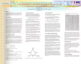
1. Parameter f2 Mean 0.65 SD 0.02 2.5% 0.62 0.68 97.5% f3 m2-m1 1.65 0.33 0.03 0.48 0.27 0.67 0.39 2.52 r1 s2a1 0.12 66 0.08 8.7 -0.04 51 0.28 85 r2 s2b1 69 0.85 9.0 0.03 53 0.80 88 0.90 s2a2 r3 0.12 82 0.09 9.0 -0.06 66 101 0.29 r4 s2b2 21 0.34 0.07 3.2 16 0.19 28 0.47 s2g1 r5 0.85 152 6.8 0.03 140 0.79 166 0.90 s2g2 f1 76 0.39 0.03 3.2 0.32 70 82 0.46 Joint Statistical Meetings New York City, August 11-15, 2002 A Bayesian Model for the Study of Accuracy, Reciprocity and Congruence in Interpersonal PerceptionParamjit GillOkanagan University College, Kelowna, BC, Canadapgill@ouc.bc.ca 2.2Bayesian Formulation The population parameters {s2a1,s2a2,s2b1,s2b2 ,s2g1 ,s2g2, r1, r2, r3, r4, r5, f1, f2, f3 }are called the variance-covariance parameters and are of primary interest. They are parts of matrices S1 = Cov(a1i,b1i,a2i,b2i) and S2 = Cov(g1ij,g1ji, g2ij,g2ji) If one does not have strong prior opinion, diffuse prior distributions for parameters and hyper-parameters can be used. Following conventional Bayesian protocol, we assume m1~ N[qm1, s2m1]; qm1 ~ N[0,10000]; s2m1~ IG[0.0001,0.0001] m2~ N[qm2, s2m2]; qm2 ~ N[0,10000]; s2m2~ IG[0.0001,0.0001] We use independent inverse-Wisharts as priors for S1 and S2 : S1-1~ Wishart4[(4I)-1,4] ; S2-1~ Wishart4[(4I)-1,4] Having specified the Bayesian model; the model assumptions and data induce a posterior distribution in accordance with the Bayesian paradigm. The posterior distribution is the distribution of the parameters conditional on the data and is the final product from which inference proceeds. Typically however, one is interested in the average value and variation of some of the parameters. If we repeatedly generate values of a parameter from the posterior distribution, average those values and calculate their standard deviation, we will then have obtained estimates of the posterior mean and posterior standard deviation. Methods of Markov chain Monte Carlo (MCMC) provide an iterative approach to variate generation from posterior distributions. Gibbs sampling algorithm (as implemented in WinBugs) is used to simulate from the marginal posterior distributions of the parameters of interest. 3.Curry & Emerson Data Example Curry & Emerson (1970) conducted a study on previously unacquainted students who lived together in a residence-hall at the University of Washington. Six 8-person round robin groups of students reported their attraction toward their group members on a 100-point scale at weeks 1, 2, 4, 6, and 8. The subjects also provided perception of attraction ratings towards them by other subjects. For simplicity, we consider five time points as replicates. A more realistic analysis would consider longitudinal profiling of variance-covariance components. Table 1 shows means, standard deviations, 2.5% and 97.5% quantiles of the marginal posterior distributions of the some key parameters for the attraction data. We see that the perception bias m2-m1 is positive but small. It means that subjects, on the average, have a pretty good idea when estimating the level of attraction they command from others. Individual level reciprocity (Mean r1 = 0.12) and its perception (Mean r2 = 0.85) make an interesting comparison. Low reciprocity means that people who are seen by others as attractive, do not see others as attractive. But people who think others as attractive assume that others think similarly about them. Individual level accuracy (Mean r4 = 0.34) is lower than the assumed individual level accuracy (Mean r5 = 0.85). This tells us that people have a poor understanding of how they are generally viewed by others. On the other hand, people assume that others have an almost perfect notion of how they are seen by others. Both the dyadic level reciprocity (Mean f1 = 0.39) and accuracy (Mean f3 = 0.33) are rather low. It is possible that these values increase with time which could be confirmed with a detailed longitudinal analysis. Not surprisingly, the dyadic congruence (Mean f2 = 0.65) is high which tells us that subjects have a tendency to like specific others because they think that those specific others like them. When compared with mean f1 = 0.39, it means that subjects believed that their unique impressions of specific partners were reciprocated more than they really were reciprocated. 2.1 Statistical Assumptions We note that SRM is a random effects model. The subjects involved in the study are assumed to be a random sample from a population and we are interested in generalizing beyond the particular persons involved in the study. Subject-specific and dyad-specific effects are assumed Normal random random variables with E(a1i) = E(a2i) = E(b1i) = E(b2i) = E(g1ij) = E(g2ij) = 0 var(a1i) = s2a1 ; var(a2i) = s2a2 ; var(b1i) = s2b1 var(b2i) = s2b2 ; var(g1ij) = s2g1 ; var(g2ij) = s2g2 Correlations among subject-specific effects represent various kinds of accuracy and reciprocity as follows.  corr(a1i ,b1i) = r1measures individual-level reciprocity of impression. A positive value means that people who are seen by others as possessing a given trait also see others as possessing the same trait.  corr(a1i ,a2i) = r2measures assumed (or perceived) individual reciprocity. A positive value indicates that people who think of others possessing a given trait also perceive that others think similarly about them. We would expect this correlation to be higher than r1which measures actual reciprocity. corr(a1i ,b2i) = r3 measures perceiver accuracy. A positive value means that perceiver’s average response (perception) well corresponds to the average impression of his interaction partners. corr(a2i ,b1i) = r4 measures individual-level accuracy. A positive value means that people have a reasonable understanding of how they are generally viewed by others as a whole. corr(b1i ,b2i) = r5 measures assumed individual-level accuracy. When people see a subject A possessing a trait (say friendly), they assume that A knows that other see him friendly. This correlation is higher than r4 which measures actual accuracy. Correlations among dyad-specific effects measure dyadic accuracy, mutuality and congruence as follows (see Figure 1). corr(g1ij ,g1ji) = f1 indicates mutuality or dyadic reciprocity in the sense that if subject A treats subject B in an especially friendly manner, does B treat A in an especially friendly manner in return? corr(g1ij ,g2ij) = f2measures dyadic congruence or assumed dyadic reciprocity in the sense that subject A likes subject B because A thinks that B likes A. corr(g1ij ,g2ji) = f3 measures dyadic accuracy of a perceiver to predict his partner’s behavior towards the perceiver. That is, if subject A sees subject B as especially friendly, does B act especially friendly with A? Table 1. Some summary results from the Bayesian analysis of attraction data Abstract A fully Bayesian approach is proposed for the analysis of accuracy and mutuality in interpersonal perceptions. The Bayesian analysis is based on social relations model (SRM) formulation. Inference is straightforward using Markov chain Monte Carlo (MCMC) methods as implemented in the software package WinBugs. An example is provided to highlight the use of Bayesian analysis of interpersonal attraction data. 1. Introduction Accuracy in interpersonal perception is a fundamental and one of the oldest topics in social and personal psychology. Are people’s perceptions of others valid? This is the most obvious question in the field of interpersonal perception, yet, surprisingly, the most difficult to study (Kenny 1994, Chapter 7). In the late 1940's and early 1950's, the study of individual differences in the accuracy of social perception became a dominant area of research but Cronbach (1955) and others argued that a comprehensive understanding of accuracy requires more sophisticated statistical and computational procedures than those available at that time. The “second wave of accuracy research” promised to provide a satisfactory solution. Kenny & Albright (1987) argued that the accuracy research must be nomothetic, interpersonal, and compartmental. They proposed the use of social relations model (SRM) as an appropriate tool to do so. Accuracy is thus defined by the links between various components of the SRM. Although the SRM provides a methodological framework for the analysis, actual practical usage is hampered by lack of available computational machinery. Purpose of this communication is to present a computationally tractable, fully Bayesian approach to the analysis of accuracy in interpersonal perceptions. The vehicle for doing this is modern Bayesian computation made accessible in the software package WinBugs (Spiegelhalter et al., 2000). The Bayesian approach is based on SRM formulation which partitions a response into various components. Accuracy is measured by interrelationships among these components. 2. Social Relations Model We follow Kenny (1994, Chapter 7) where social relations model is proposed to for the study of accuracy of personal perceptions. We assume that the design used in the study is round robin or reciprocal. That is, each subject serves as judge and target and each subject interacts with all other subjects. For each dyad (pair) of subjects i and j, we have four measurements on the level of a trait yij, yji, xij and xji. Here yij represents the response (impression) of subject i as an actor (judge) towards subject j as a partner (target) and xji represents a postdiction (perception) by partner j of the impression yij. In yjiand xij the roles are reversed. The SRM partitions the responses into population-specific, actor-specific, partner-specific and dyadic components in an additive fashion yij = m1 + a1i+ b1j+g1ij xji = m2 + a2j+ b2i+g2ji yji = m1 + a1j+ b1i+g1ji xij = m2 + a2i+ b2j+g2ij The model parameters are divided into three groups Population-specific: m1 = population average impression m2 = population average perception m2 - m1= Perception bias the subjects have in estimating their own trait level Subject-specific: a1i=average impression that subject i has about others a2i= average perception that subject i has about what others think of him b1i= average impression others have of subject i b2i = average perception others have of subject i’s impression of others Dyad-specific: g1ij= dyadic interaction between subjects i and j as reported by i as a judge. It is the special relative impression of i toward j, subtracting out the actor and partner effects. g2ji= perception by subject j of the dyadic interaction g1ij Among the variance components, we find that actor and partner variations in attraction levels are very similar (Mean s2a1 = 66,Mean s2b1= 69). It is, however, interesting to note that there is substantial actor variation in perception (Mean s2a2 = 82). It tells us that some people believe that they are more attractive and others believe that they are not that attractive. On the other hand, partner variation in perception is relatively much lower (Mean s2b2 = 21). That is, there is a slight tendency for some people to be seen as harsh judges and others to be seen as lenient ones. The dyadic variance in the reported attraction level (Mean s2g1 = 152) is almost double than the dyadic variance in the perceived attraction (Mean s2g2 = 76). It tell us that subjects were not capable of fully realizing the extent of variability in dyadic interactions. 4. Future Research The relationship between persons develops over time and therefore, the model should accommodate the longitudinal nature of data. It means that the model parameters are assumed to be occasion-specific. It would be of interest to include covariates (such as sex) in the model. For example, in the Curry-Emerson study, the students lived in the residences as room-mate pairs. Work on measuring the effect of physical proximity on the degree of accuracy, reciprocity and congruence is under progress. 5. References 1. Cronbach, J. L (1955). Psychological Bulletin, 52, 177-193. 2. Curry, T.J. & Emerson, R.M.(1970). Sociometry, 33, 216-238. 3. Kenny, D.A.(1994). Interpersonal Perceptions. Guilford Press: New York 4. Kenny, D.A. & Albright, L.(1987). Psychological Bulletin, 102, 390-402. 5. Spiegelhalter, D., Thomas, A. & Best, N.(2000). WinBUGS User Manual. MRC Biostatistics Unit: Cambridge. 6. Acknowledgements This research is being supported by a grant from the Natural Sciences and Engineering Research Council (NSERC) of Canada and is a part of ongoing joint work with Professor C. F. Bond Jr. of Texas Christian University, Fort Worth. Figure 1. Mutuality, congruence, and accuracy triangle (Kenny & Albright, 1987)