Research Objectives

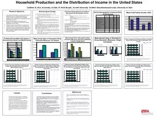
1. Household Production and the Distribution of Income in the United StatesCathleen D. Zick, University of Utah, W. Keith Bryant, Cornell University Sivithee Srisukhumbowornchai, University of Utah Research Objectives • Use the 2003 ATUS data to examine the impact of adding the value of household production to money income to arrive at a more complete measure of the distribution of household economic well-being in the U.S. • Assess how sensitive the estimates are to variations in the definition of housework and the measurement of its value. • Compare the income distribution implications for married couples, single women, and single men. • Contrast the results obtained with the 2003 data to earlier work done by Bryant and Zick (1985) and Zick and Bryant (1990) using the Panel Study of Income Dynamics. Methodological Strategy Mean Total Family Income: 2002 ATUS 2003 Sample Matched to the March 2003 Social and Demographic Survey Socio-Demographic Characteristics of the Sample • Use two alternative measures of time spent in housework • Core housework as defined by the ATUS Lexicon • Housework as defined by Margaret Reid (1934) (i.e., ATUS core housework plus time spent shopping and time spent in child care) • Use two alternative measures of the economic value of an hour of housework • Opportunity cost measure based on the predicted after-tax wage rate. These predicted after-tax wage rates are obtained from regressions that correct for sample selection bias (Heckman, 1979) and are estimated separately by gender and marital status. • Replacement cost measure based on the median before-tax wage rate for individuals in the March 2003 CPS who reported that their primary occupation was housekeeper/maid. • Only one individual (age 15+) in each household was selected to complete the 24-hour time diary. In households with more than one adult, this would lead to an underestimation of the total household production time. We will follow the imputation methods used by Bonke (1992) to remedy this issue. • Time spent in housework over a synthetic year is constructed by: • Estimating housework tobits separately by gender and marital status & controlling for socio-demographic covariates including whether or not the diary came from a weekday or weekend. • Using these tobits to generate predicted time spent in housework for a weekday and a weekend day. These estimates are then used to create a predicted measure of time spent in housework for the year. • Selection Criteria: • white non-hispanic, black non-hispanic, and hispanic respondents, • respondents living with a spouse/partner or living as a single head of household, and • Who were in the March 2003 Social and Demography Survey • Sample Size: 5,623 • 3,444 married couples • 1,398 single females • 781 single males • Income and wage information were taken from the March 2003 Social and Demographic Survey • Time spent in housework for the respondent and socio-demographic information for the respondent and his/her spouse were taken from the 2003 ATUS. • The median replacement wage rate, $7.36/hr, was generated from the March 2003 Social and Demographic Survey (weighted) for individuals who reported their primary occupation to be housekeeper/maid (N=1,120, excluding the top and bottom 1%). • All estimates that made use of the time diary data were weighted using the 2003 ATUS weight. Predicted Annual Mean Time Spent in Housework by Gender and Marital Status Mean Annual Value of Housework Using Alternative Measures: Full Sample Mean Annual Value of Housework Using Alternative Measures: Married/Cohabitating Couples Disaggregated Mean Annual Value of Housework Using Alternative Measures: Single Individuals Relative Economic Well-Being as Measured by Money Income Plus the Dollar Value of Housework: Full Sample* • P10/P50 P90/P50 P90/P10 • (Low Income) (High Income) (Decile Ratio) • 36 215 602 • 224 720 • 226 667 • 227 728 • 28 254 934 Hrs/Yr Single Men Single Women % *Length of bars represents the gap between high and low income households. Numbers in the first two columns of the table are the percent of median household income. Numbers in the last column of the table represent the 90th percentile income as a percent of the 10th percentile income. The graph and table presented here are based on the income distribution approach used Garfinkel, Rainwater, and Smeeding (2005). Relative Economic Well-Being as Measured by Income Plus the Dollar Value of Housework: Married/Cohab Couples* Relative Economic Well-Being as Measured by Money Income Plus the Dollar Value of Housework: Single Women* Relative Economic Well-Being as Measured by Money Income Plus the Dollar Value of Housework: Single Men* Relative Economic Well-Being as Measured by Money Income Plus the Dollar Value of Housework: The Contributions of Husbands in Married Couple Households* Relative Economic Well-Being as Measured by Money Income Plus the Dollar Value of Housework: The Contributions of Wives in Married Couple Households* • P10/P50 P90/P50 P90/P10 • (Low Income) (High Income) (Decile Ratio) • 50 195 389 • 45 198 433 • 46 206 446 • 43 204 467 • 33 229 686 • P10/P50 P90/P50 P90/P10 • (Low Income) (High Income) (Decile Ratio) • 41 214 521 • 40 212 529 • 39 218 565 • 38 218 572 • 33 229 686 • P10/P50 P90/P50 P90/P10 • (Low Income) (High Income) (Decile Ratio) • 52 222 626 • 44 229 518 • 48 237 490 • 44 242 551 • 34 266 777 • P10/P50 P90/P50 P90/P10 • (Low Income) (High Income) (Decile Ratio) • 37 231 627 • 36 236 664 • 36 237 657 • 34 235 692 • 28 247 871 • P10/P50 P90/P50 P90/P10 • (Low Income) (High Income) (Decile Ratio) • 45 205 452 • 42 208 491 • 43 214 496 • 41 214 525 • 33 229 686 % % % % % *Length of bars represents the gap between high and low income households. Numbers in the first two columns of the table are the percent of median household income. Numbers in the last column of the table represent the 90th percentile income as a percent of the 10th percentile income. The graph and table presented here are based on the income distribution approach used Garfinkel, Rainwater, and Smeeding (2005). *Length of bars represents the gap between high and low income households. Numbers in the first two columns of the table are the percent of median household income. Numbers in the last column of the table represent the 90th percentile income as a percent of the 10th percentile income. The graph and table presented here are based on the income distribution approach used Garfinkel, Rainwater, and Smeeding (2005). *Length of bars represents the gap between high and low income households. Numbers in the first two columns of the table are the percent of median household income. Numbers in the last column of the table represent the 90th percentile income as a percent of the 10th percentile income. The graph and table presented here are based on the income distribution approach used Garfinkel, Rainwater, and Smeeding (2005). *Length of bars represents the gap between high and low income households. Numbers in the first two columns of the table are the percent of median household income. Numbers in the last column of the table represent the 90th percentile income as a percent of the 10th percentile income. The graph and table presented here are based on the income distribution approach used Garfinkel, Rainwater, and Smeeding (2005). *Length of bars represents the gap between high and low income households. Numbers in the first two columns of the table are the percent of median household income. Numbers in the last column of the table represent the 90th percentile income as a percent of the 10th percentile income. The graph and table presented here are based on the income distribution approach used Garfinkel, Rainwater, and Smeeding (2005). Caveats References Conclusions • Bonke, J. 1992. “Distribution of economic resources: Implications of including household production.” Review of Income and Wealth, 38, 281-293. • Bryant, W. K. And C.D. Zick. 1985. “Income distribution implications of rural household production.” American Journal of Agricultural Economics, 65, 1100-1104. • Garfinkel, I. L. Rainwater, and T.M. Smeeding. 2005. “Welfare state expenditures and the redistribution of well-being: Children, elders, and others in comparative perspective.” Working Paper, Syracuse University. • Heckman, J.J. 1979. “Sample selection bias as a specification error.” Econometrica 47, 153-161. • Reid, M.G. 1934. Economics of Household Production. New York: John Wiley. • Zick, C. D. And W. K. Bryant. 1990. “Shadow wage assessments of the value of home production: Patterns from the 1970s.” Lifestyles: Family and Economic Issues, 11, 143-160. • Estimation of housework is based on a single diary day. From these single day diaries, we constructed a synthetic year of housework making adjustments for weekday and weekend differences. • Estimates for respondents’ spouses were imputed. • Estimates are based on reports of primary time spent in housework. No secondary housework time was included. As such, these are lower-bound estimates. • Because of the need to match to the March Social and Demographic Supplement, no observations were drawn from the winter quarter. To the extent that housework time differs between winter and the other three seasons, we were not able to control for this factor. • The 2003 ATUS reveals that large amounts of time are being spent in core (expanded) housework. At one extreme, married women average approximately 21 (35) hrs/wk. At the other extreme, single men average 8 (12) hrs/wk in core (expanded) housework. • Estimates of the annual average economic contribution of housework range from $10,128 (core housework using replacement costs) to $23,994 (expanded housework using opportunity costs). Clearly, the economic contributions of housework are substantial. • The largest contributions typically occur in married/cohabitating couple households with wives typically contribute the most. This holds for every estimation approach. • Similar to Bryant and Zick (1985) and Zick and Bryant (1990), we find a modest decrease in the income distribution range when the economic value of housework is added to money income. This finding holds regardless of which measure we use. • The largest gains in terms of decreasing income inequality occur for married/cohabitating couples and single women. Single men experience smaller gains in income equality.