Download
1 / 53
530 likes | 683 Views
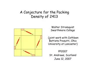
A Conjecture for the Packing Density of 2413. Walter Stromquist Swarthmore College (joint work with Cathleen Battiste Presutti, Ohio University at Lancaster) PP2007 St. Andrews, Scotland June 12, 2007. Outline. 1. About packing densities 2. Packing rates for measures:

E N D
A Conjecture for the Packing Density of 2413 Walter Stromquist Swarthmore College (joint work with Cathleen Battiste Presutti, Ohio University at Lancaster) PP2007 St. Andrews, Scotland June 12, 2007
Outline • 1. About packing densities • 2. Packing rates for measures: • a. There is an optimal measure for every pattern • b. Packing rate = Packing density • 3. An optimal measure for 2413: • the best we can do without recursion • 4. Amazing things happen with recursion bubbles • 5. Conjecture for 2413: 0.10472422757673209041…
About packing densities… • A pattern is a permutation in Sm. • Let n Sn. An occurrence of in n is an m-element • subsequence of n that has the same order type as . • reduces to . • Define • The packing density of in n is • Clearly,
About packing densities… • We’re concerned with permutations nSn that maximize the • packing density ( , n ). So, define: • Any permutation n* that achieves this maximum (for a given • size n) is called an optimizer for (or, optimizing permutation). • The packing density of is the limiting value, • (It always exists.)
About packing densities… • Equivalently: The packing density of is the largest number D • such that there is a sequence of permutations • of increasing size such that • The n ‘s don’t have to be optimizers; they just have to be close enough that they have the right limit.
Describing the near-optimizers • Here’s how we describe good n‘s for 132: That’s what the n‘s look like. The packing density turns out to be
Describing the near-optimizers • Here’s an easier picture: The points line up along these lines. This object is a probability measure on the unit square. Let’s formalize it.
Measures on the Unit Square • Let S be the unit square, • S = [0, 1] [0, 1] R2. • A probability measure on S is a probability distribution on S. • If a point is selected randomly according to , then (A) is the probability that the point is in A. is non-negative and countably additive. Also, (S) = 1. All measures in this talk are probability measures on S.
The packing rate for a measure • Let m be a pattern, and let be a measure. • If m points are selected randomly according to , then the packing rate of with respect to is the probability that the order type of their configuration is . • We denote this packing rate by ’ ( , ) . • More precisely: Let m = … be the product measure on S m = S S … S. Let A Sm contain all m-tuples of points that form configurations with order type . Then • ’ ( , ) = m ( A ).
“…order type of their configuration…” If the points are ordered by increasing x coordinates, x1 < x2 < … < xm, then the order type of the configuration is the order type of their y coordinates ( y1, y2, …, ym ). The order in which the points are selected is irrelevant. If any two points have the same x coordinate or the same y coordinate, then the configuration has no order type. These four points have order type 2314.
Examples of packing rates • Example. Let be the uniform measure on S. • Then all order types are equally likely. We therefore have • ’ ( 123, ) = 1/6 • and, in general, • ’ ( , ) = 1 / m! • if has size m. Points are drawn uniformly from the unit square.
Examples of packing rates • Example. Let be concentrated along the main diagonal. • Then • ’ ( 123, ) = 1 • and • ’ ( , ) = 0 • for any other pattern of size 3. It doesn’t matter how probability is distributed along the diagonal.
Examples of packing rates • Example. Let be concentrated along countably many diagonal segments as shown. • Then • ’ ( 132, ) = • This is the packing density of 132. No other measure gives a higher packing rate for 132. This is the “optimal measure” for 132.
Examples of packing rates • Example. Let be uniform • on a disk in S. • WHAT IS ’ ( 123, ) ? Points are drawn uniformly from the disk.
Optimal Measures • Given a pattern , the optimal packing rate of (or just the packing rate of ) is • ’() = ( ’ (, ) ) • where the supremum is taken over all measures. • Any measure that realizes the supremum is called an optimal measure for . • Does every pattern have an optimal measure ? YES.
Optimal Measures • Is there always an optimal measure? • Why not just find measures i whose packing rates approach the maximum, and take the limiting measure? • (1) It’s tricky to define limiting measures • (2) Limits of measures don’t always preserve packing rates
Limits of measures • If i is a measure for each i and is a measure, we say that • = lim i • if • for every continuous function f on S. • With this definition, the set of probability measures on S forms a compact topological space. • So, for any sequence {i} of measures, there is a subsequence {i} with a limit = lim i. • But the packing density of is not always equal to the limit of the packing rates of the i’s.
n is concentrated on [ 1/(n+1), 1/n ]2 is a point mass at the origin Example – limits don’t preserve packing rates • In this picture, = lim i. • But ’ ( 132, i ) = 1/6 for each i, while ’ ( 132, ) = 0.
Normalized Measures • A measure on S is normalized if its projections on both • the x and the y axis are uniform distributions. • A limit normalized measures is normalized. • If the measures i are all normalized and = lim i then • ’ ( , i ) = lim ’ ( , i ) . • Every measure can be normalized by monotone transformations of the x and y coordinates. This operation can’t reduce packing rates.
Every pattern has an optimizing measure • Theorem: For every pattern , there is a measure such that • ’ (, ) = ( ’ (, ) ) = ’() . • The measure can be chosen to be normalized. • Proof: Pick measures {i} whose packing densities approach the supremum. Replace them with normalized measures {i}. Find a subsequence that converges to a limit measure . Then is normalized, and is an optimizing measure for . // • Question: Is the normalized optimal measure for always unique? • (Probably not, but it would be very nice if it were.)
Packing rates = Packing densities • Theorem: The optimal packing rate of any pattern is its packing density: • ’ ( ) = ( ).
Packing rates = Packing densities • Why ( ) ’ ( ) : • Given any measure , just pick n randomly according to . Then on average the packing rate of in n is exactly ’ (, ). • So, we can pick particular n‘s that achieve this average, and then we have • lim ( , n ) = ’ ( , ). • This forces ( ) ’ ( ) .
Packing rates = Packing densities • Why ’ ( ) ( ) : • Find a sequence of measures n with lim ( , n ) = ( ). • For each n , construct a template measure (Presutti, PP2006): • Now the limit of the template measures (or of some subsequence of them) is a measure with ’ ( , ) = ( ). • So ’ ( ) ( ).
Summary • For every pattern , there is a normalized optimizing measure that maximizes ’ ( , ). • For that measure, ’ ( , ) = ( ). • So, to find the packing density, it suffices to find an optimizing measure.
About 2413… • Why 2413 ? • (1) Least-understood pattern of size 3 or 4 • (2) As far as possible from being layered • What we know… • ( 2413 ) 6/64 = 0.09375 (because that bound • works for any of size 4) • ( 2413 ) 51/511 = 0.099804… (AAHHS, template of size 8) • ( 2413 ) 0.104250980… (Presutti, weighted template • of size 16) • Upper bound: • ( 2413 ) 2/9 (AAHHS, not likely tight) • Today’s conjecture: • ( 2413 ) ≈ 0.10472422757673209041…
An optimal measure for 2413 ? • So, what is an optimal measure for 2413? • By symmetry and computational experience, we suspect a measure of this form:
Probability distribution along this line: F(t) F(t) = fraction of this segment’s probability that is in the leftmost fraction t of the segment t=0 ……………………….t=1
Symmetrical Four-Segment Measures • (1) Probability is concentrated along the four segments shown • (2) Measure has four-fold rotational symmetry • (3) Measure is partially normalized … combined mass of top and • bottom segments is uniform on [1/4, 3/4], and similarly for • side segments • F(t) + ( 1 – F(1-t) ) = 2t for t in [0, 1] • Values of F on [0, ½] determine all of F
Examples of Symmetrical Four-Segment Measures • Example: F(t) = t (for all t) --- probability is uniform along • all four segments. • packing rate is 6/64. (Not obvious!) • Example: F(t) = 0 for t in [0, ½], • 2t-1 for t in ( ½, 1] --- probability is uniform • along outer half of each segment • packing rate is 6/64 ( four points form an instance • of 2413 iff one point is on each segment )
Examples of Symmetrical Four-Segment Measures • Example:F(t) has slope 0 in [ 0, ¼ ] and [ ½, ¾ ] • slope 2 in [ ¼ , ½ ] and [ ¾, 1 ]. • packing rate is 51/512 • ( this is essentially the AAHHS estimate )
Examples of Symmetrical Four-Segment Measures • Example: F(t) = t2 for t in [0, 1] • packing density = 349/3360 ≈ 0.103869… • (Better than 51/511 ≈ 0.099804…, • but not as good as the current record) • …This shows that there may be some advantage to an uneven distribution.
Packing rate calculated from F… • Theorem. Let be a symmetrical four-segment measure with the distribution along each segment given by F. • Then the packing rate is given by
How would one prove such a formula? • There are three possibilities for 2413-patterns arising from : One point per segment Two, one, one Two pairs …works only if right dot is above left dot, and bottom dot right of top dot
Chance of getting type 1 • Probability of an occurrence of the first • type: • (1) Probability that points are in four • different segments: 6/64 • (2) Probability that right point is above • left point:
Chance of getting type 1 • (3) Probability that bottom point is to • right of top point: Same as (2) • (4) Therefore: Probability of type 1 • occurrence of 2413: • Calculate type-2 and type-3 probabilities similarly; add to get theorem.
Calculus of Variations • Write: • How do we choose F to maximize this value ? • Theorem: Let . If F maximizes the expression above, then • whenever F is not constrained at t. • (That is, whenever the slope of F is not 0 or 2.)
So what is F ? • The above formula gives a negative value when t < ¼ - 2J. So the real formula is • F(t) = 0 if t < t* = ¼ - 2J, • = formula above if t t* • The above formula makes F dependent on J, which is an integral of F itself. The resulting condition determines J and t*: • t* ≈ 0.14779091617675321550… • J ≈ 0.05110454191162339225…
So what is F ? • …so finally, F(t) is given by • F(t) = 0 when t < 0.14779091617675321550… • otherwise.
Best packing rate ? • This F gives • ’ ( , ) ≈ 0.10472339512772223636… • which is a new lower bound for the packing density of 2413. • Compare last year’s value, from weighted template: 0.104250980…
Recursion bubbles • But wait! • This plan leaves about 14% of each segment empty.
With the recursion bubble… • Recall packing rate so far: 0.10472339512772223636… • With one recursion bubble on each segment, the packing rate becomes… • 0.10472417578055968289… • …A MASSIVE IMPROVEMENT !
Shouldn’t the recursion bubble be bigger? • Shouldn’t it? The measure was optimal before we introduced recursion. Now, there’s more advantage to drawing points from the box than there was before. At the margin, isn’t that a reason for increasing the size of the bubble? • So, make the bubble bigger. • But then the low end of F is inconsistent. We need to add another recursion bubble to get F back on track. • And then another, and another, and another…