Chapter 2

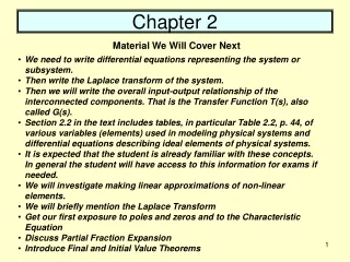
1. Chapter 2 Material We Will Cover Next • We need to write differential equations representing the system or subsystem. • Then write the Laplace transform of the system. • Then we will write the overall input-output relationship of the interconnected components. That is the Transfer Function T(s), also called G(s). • Section 2.2 in the text includes tables, in particular Table 2.2, p. 44, of various variables (elements) used in modeling physical systems and differential equations describing ideal elements of physical systems. • It is expected that the student is already familiar with these concepts. In general the student will have access to this information for exams if needed. • We will investigate making linear approximations of non-linear elements. • We will briefly mention the Laplace Transform • Get our first exposure to poles and zeros and to the Characteristic Equation • Discuss Partial Fraction Expansion • Introduce Final and Initial Value Theorems

2. Control Systems are Often More Complex Than Single Loops • One forward path • Four transfer functions in the forward path G1, G2, G3, G4. • Three Feedback Loops. • Three Summing Junctions

3. H3 1 G3 1 C(s) 1 G1 G2 G4 R(s) -H2 -H1 Block Diagram = Flow Graph Besides Block diagrams, control systems are often represented using Flow Graphs Block Diagram Flow Graph Note that two of the H transfer functions in the Flow Graph have negative signs. This is necessary since the summing nodes do not have any signs associated with them as in the block diagram.

4. R(S) + E C(s) G1 _ F H Solve For The Transfer Function • Solution: • C(s) = G1E (1) • F = C(s)H (2) • E = R(s)-F (3) • E = R(s)-C(s)H (4) • C(s) = G1[R(s)-C(s)H] (5) • C(s) +C(s)HG1 = G1(R(s) • C(s)[1 + HG1] = G1(R(s) • C(s)/R(s)=G1/(1+G1H)

5. A G1 + C(s) + R(S) + B E G2 _ F H Solve For The Transfer Function • Solution: • C(s) = A + B (1) • A = G1E (2) • B = G2E (3) • F = HB (4) • E = R(s)-F (5)

6. Attempt to Solve For The Transfer Function D A B E F J M C K

7. Overall Transfer Function Mason’s Gain Rule The overall Transfer function can be obtained from the formula: • Mk is the transmittance of each forward path between a source and a sink node • ∑L1 is the sum of the transmittances of each closed path. • ∑L2 is the sum of the product of the transmittances of all possible combinations of two non-touching loops. • ∑L3 is the sum of the product of the transmittances of all possible combinations of three non-touching loops. • ∆k is the cofactor of Mk. It is the determinant of the remaining sub-graph when the forward path which produces Mk is removed. Thus it does not include any loops which touch the forward path in question. It is equal to unity when the forward path touches all the loops in the graph of when the graph contains no loops.

8. H3 1 G3 1 C(s) 1 G1 G2 G4 R(s) -H2 -H1 Applying Mason’s Gain Rule

9. G9 -H2 G5 G2 G6 G1 G8 G3 G7 G4 R(s) C(s) -H4 -H5 -H1 -H3 Applying Mason’s Gain Rule

10. 1 1 G3 C R B G1 1 G4 G2 A 1 -1 -1 -1 Using Mason’s Gain RuleSolve for the Transfer Function – C/R

11. 1 1 G3 C R B G1 1 G4 G2 A 1 -1 -1 -1 Applying Mason’s Gain Rule

12. C(s) Manipulated Variable + R(s) Error - Feedback H = 0.5 Derive Transfer Function for Previous Control System Example Note: The denominator, set equal to zero, is called the Characteristic Equation

13. b K Output = y(t) Input = f(t) Process Block Diagram M y f F(s) Y(s) F(s) Y(s) General Quadratic Form F(s) Y(s) Spring Mass System Block Diagram

14. F(s) Y(s) F(s) Y(s) General Quadratic Form F(s) Y(s) More on the Characteristic Equation Block Diagram

15. jω x 4 4 -6 -5 -4 -3 -2 -1 x -4 Characteristic Equation • The denominator polynomial of the transfer function when set equal to zero is called the characteristic equation C.E.. • The roots of the C.E. are the poles of the system. • The roots of the transfer function’s numerator are the zeros of the system. • Poles and zeros are critical frequencies • At the poles, the transfer function becomes infinite • At the zeros the transfer function becomes zero. • The complex frequency s-plane plot of the poles and zeros graphically portrays the character of the natural transient response of the system.

16. Any time the roots are equal and real, the system is critically damped, no overshoot. Double Root X • Any time the roots are unequal and real, the system is overdamped, no overshoot. X X jω jω Root Location vs Stability of the 2nd order C.E.

17. Anytime the roots are complex conjugates, the system experiences damped oscillation X X • If the poles lie on the imaginary axis the system is marginally stable. It oscillates. X X jω jω Root Location vs Stability of the 2nd order C.E.Continued

18. jω X X jω X X Root Location vs Stability of the 2nd order C.E.Continued • Anytime the roots are in the RHP the system is unstable and diverges

19. J, b Ra La ea em Ia ө, ω Deriving a Transfer Function for a Control System ComponentConsider a DC Torque Motor J = Motor Inertia, could also include load inertia b = Friction Ra = Motor winding resistance La = Motor inductance em = Back emf KT = Motor Torque Sensitivity – A motor parameter Km = Relates back emf to shaft speed, em = Kmω

20. J, b Ra La ea em Ia ө, ω Deriving a Transfer Function for a DC Torque MotorContinued KVL around loop: Motor and Load Inertia Equations (1), (2), (3), and (4) are called Equilibrium Equations

21. Ia(s) Ia(s) Ia(s) Ia(s) Tm(s) Tm(s) Tm(s) Tm(s) KT KT KT KT Em(s) Kms Ea - Em Ea(s) + - Em(s) Kms Constructing Block Diagram for a DC Torque MotorFrom Equilibrium Equations

22. Ia(s) Tm(s) KT Ea - Em Ea(s) + - Em(s) Kms Constructing DC Motor Transfer Function from Block Diagram Using Mason’s Rule