Random Effects Analysis
Random Effects Analysis. Will Penny. Wellcome Department of Imaging Neuroscience, University College London, UK. SPM Course, London, May 2004. ^. ^. ^. ^. ^. 11. 12. . 1. 2. ^. ^. ^. ^. 2. 12. 1. 11. Summary Statistic Approach.

Random Effects Analysis
E N D
Presentation Transcript
Random Effects Analysis Will Penny Wellcome Department of Imaging Neuroscience, University College London, UK SPM Course, London, May 2004
^ ^ ^ ^ ^ 11 12 1 2 ^ ^ ^ ^ 2 12 1 11 Summary Statistic Approach 1st Level 2nd Level DataDesign MatrixContrast Images SPM(t) One-sample t-test @2nd level
Validity of approach • Gold Standard approach is EM – see later – estimates population mean effect as MEANEM the variance of this estimate as VAREM • For N subjects, n scans per subject and equal within-subject variance we have VAREM = Var-between/N + Var-within/Nn • In this case, the SS approach gives the same results, on average: Avg[a] = MEANEM Avg[Var(a)] =VAREM ^ ^ Effect size
Example: Multi-session study of auditory processing SS results EM results Friston et al. (2004) Mixed effects and fMRI studies, Submitted.
Two populations Estimated population means Contrast images Two-sample t-test @2nd level Patients Controls One or two variance components ?
The General Linear Model y = X + e N 1 N L L 1 N 1 Error covariance N 2 Basic Assumptions • Identity • Independence N
y = X + e N 1 N L L 1 N 1 Multiple variance components K =1 Error covariance N Errors can now have different variances and there can be correlations N K=2
y = X + e N 1 N L L 1 N 1 ( ) - 1 - = T 1 C X C X e q E-Step y - h = T 1 C X C y e q q y y for i and j { = - h r y X q y M-Step - - - - - = - - 1 T 1 1 T 1 1 g tr { Q C } r C Q C r tr { C X C Q C X } e e e e e q i i i i y - - = } 1 1 J tr { Q C Q C } e e ij j i - l = l - 1 J g å = + l C C Q e q k k Estimating variances EM algorithm Friston, K. et al. (2002), Neuroimage
Example I U. Noppeney et al. Stimuli:Auditory Presentation (SOA = 4 secs) of (i) words and (ii) words spoken backwards Subjects: (i) 12 control subjects (ii) 11 blind subjects jump Eg. “Book” and “Koob” touch “click” Scanning: fMRI, 250 scans per subject, block design
Population Differences Controls Blinds 1st Level 2nd Level } Contrast vector for t-test Covariance Matrix } Design matrix Difference of the 2 group effects