Download
1 / 32
450 likes | 1.11k Views
Signal Energy & Power. MATLAB HANDLE IMAGE USING single function with 3 Dimensional Independent Variable, e.g. Brightness(x,y,colour). Signal Energy & Power. Border or Edge. Signal Energy & Power. Signal Energy & Power. Signal Energy & Power. Signal Energy & Power.

E N D
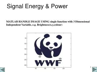
Signal Energy & Power MATLAB HANDLE IMAGE USING single function with 3 Dimensional Independent Variable, e.g. Brightness(x,y,colour)
Signal Energy & Power Border or Edge
Signal Energy & Power Instantaneous Power Dissipated By Resistor R ohms. Total energy expanded over time interval between t1 and t2 is :-
Average Power Similarly for the automobile , instantaneous power dissipated through friction is:-
Energy over infinite interval Let us examine energy over the time interval or number of sample that is infinite:-
Infinite energy • If x(t) or x[n] equals a nonzero constant value for all time or sample number, the integral or summation will not converged, therefore the energy is infinite. • Otherwise it will converge and the energy will be finite if x(t) or x[n] tends to have zero values outside a finite interval.
Time-average power over infinite interval With this 3 classes of signals can be identified:- 1) Finite total energy, 2) Finite average power, 3) Neither power nor energy are finite,
Finite total energy signal. -5 < n <+5, x[n] = 1 otherwise x[n]=0. ENERGY =11.
Finite average power x[n] = 4, for all n. ENERGY =infinite, Power = 16
Neither power nor energy are finite X[n]=0.5n, for all n.
Transformation of Independent Variable. • Central concept in signal & system is the transformation of a signal. • Aircraft control system:- • Input correspond to pilot action • these action are transformed by electrical & mechanical system of the aircraft to changes to aircraft trust or position control surfaces such as the rudder & ailerons. • finally these changes affect the dynamics & kinematics such as the aircraft velocity and heading.
High fidelity audio system • Input signal representing music recorded on cassette or compact disc. • This signal is modified or transformed to enhanced the desirable characteristics. • Such as, remove recording noise and to balance the several components of the signal e.g. treble and bass.
Modification of independent variable (time axes) • Introducing several basic properties of signals & systems through elementary transformations. • Examples of elementary transformation:- • time shift, x(t-t0), x[n-n0] • time reversal, x(-t), x[-n]. • time scaling, x(0.5t), x[2n]. • and combinations of these. x(at+b), x[an-b], where a & b are signed constants*.
Shifting right or lagging signal x(t) X(t) 0 t X(t-t0) t t0 0 is a positive value
Shifting left or leading signal x(t) X(t) 0 t X(t+t1) t -t1 0
Time scaling of continuous signal x(t) t x(2t) Compression a>1 t x(t/2) Linearly stretching a<1 t
Examples x[n] x[n-5]
Examples x[n] x[n+5]
Examples x[n] x[-n+5]
Example 1.1 x(t) 1 1 t 0 2 x(t+1), x(t) shifted left by 1sec 1 -1 0 1 2 t
Tables of x(t) & x(t+1) & x(-t+1) t x(t) x(t+1)x(-t+1) -2 0 00 -1 0 10 0 1 11 1 1 01 2 0 00 3 0 00
Example 1.1 x(t+1) is x(t) shifted left by 1 1 1 -1 t 0 2 x(-t+1) is x(t+1) flipped about t=0 1 -1 0 1 2 t
Example 1.1 Alternative 1 x(t-1) is x(t) shifted right by 1sec 1 1 t 0 2 1 x(-t+1)=x(-1(t-1)) Flip about axis t=1 -1 0 1 2 t
Example 1.1, Method 2 x(-t), flip about axis t=0 1 -1 t 0 1 2 x(-t+1), shift right (because -t) by 1 1 -1 0 1 2 t
Example 1.1 x(t) 1 1 t 0 2 x(t+1), x(t) shifted left by 1sec 1 -1 0 1 2 t
Example 1.1 x(3t/2), x(t) compressed by 2/3 1 -1 0 1 2 t 2/3 4/3 x((3/2)*(t+2/3)), x(t) compressed by 2/3 & shifted left by 2/3 1 -1 0 1 t -2/3 2/3