Download
1 / 32
350 likes | 605 Views
Application of “blind” deconvolution to Adaptive Optics Imaging. Julian C. Christou Center for Adaptive Optics. Adaptive Optics Imaging. Quality of compensation depends upon: Wavefront sensor Signal strength & signal stability

E N D
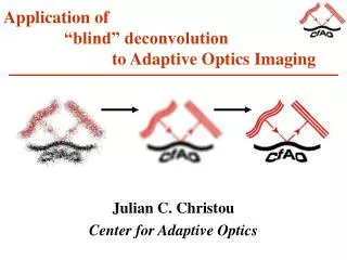
Application of “blind” deconvolution to Adaptive Optics Imaging Julian C. Christou Center for Adaptive Optics
Adaptive Optics Imaging • Quality of compensation depends upon: • Wavefront sensor • Signal strength & signal stability • Speckle noise (d / r0) • Duty cycle (t / t0) • Sensing & observing λ • Wavefront reconstructor & geometry • Object extent • Anisoplanatism (off-axis)
Adaptive Optics Imaging Poorly compensated image (SR ~ 5%) (200 msec) Uncompensated image (200 msec)
Adaptive Optics Point Spread Function Variability • Differences in Target & Reference compensation due to: • Temporal variability (changing r0 & t0). • Object dependency (extent and brightness) • full & sub-aperture tilt measurements • Spatial variability • Adaptive Optics PSFs are poorly determined.
The Imaging Equation Shift invariant imaging equation (Image & Fourier Domains) g(r) = f(r) * h(r) + n(r) G(f) = F(f) • H(f) + N(f) g(r) – measurement h(r) – Point Spread Function (blur) f(r)– Target
Physically Constrained Iterative Deconvolution • “Blind” deconvolution solves for both objectf(r) and PSF h(r) simultaneously. • Ill-posed inverse problem. • Under – determined: 1 measurement, 2 unknowns • Uses Physical Constraints. • f(r) & h(r) are positive, real & have finite support. • Finite support reduces # of variables (symmetry breaking) • h(r) is band-limited – symmetry breaking • a priori information - further symmetry breaking. • Noise statistics • PSF knowledge • Object & PSF parameterization • Multiple Frames: • Same object, different PSFs. • N measurements, N+1 unknowns.
idac – iterative deconvolution algorithmin c • Developed at Steward Observatory • Authors – Keith Hege, Matt Chesalka • Collaborators - Stuart Jefferies & Julian Christou • Available to download from SO & CfAO • http://babcock.ucsd.edu/cfao_ucsd/idac/idac_package/idac_index.html • http://bach.as.arizona.edu/~hege/docs/idac.html • “blind” and fixed PSF multi-frame deconvolution
idac – iterative deconvolution algorithmin c • Conjugate Gradient Error Metric Minimization E = Econv + Ebl +ESAA • Convolution Error Econv = ik[gik – (f 'i * h'ik)]2 • Band-limit Error Ebl = k u > uc|H'uk|2 • Non-negativity f 'i = 2& h'ik = 2 • PSF Constraint ESAA = i|hiSAA – h'iSAA|2
idac – iterative deconvolution algorithmin c • Regularization via Truncated Iterations Econv = ik[(gik + nik) – (f 'i * h'ik)]2 = ik |nik |2 = kn2 • SNR Regularization (Fourier Domain) Econv = uk[Guk – (F'u• H'uk)]2 u u = (| Gu|2 - |Nu| 2) / | Gu|2
Applications of “idac” to AO Data 1. Solar System Objects • Keck AO imaging of Uranus’ Rings • ADONIS Imaging of Io • Starfire Optical Range • Artificial Satellite • Close Binary Stars • Gemini/Hokupa’a Imaging of the Galactic Center Using Starfinder for Photometry and Astrometry
Keck AO Imaging of Uranus Observations (Imke de Pater - UCB) Keck II AO • = 2.2 m Loop closed on Uranus 3 frames/data set 90° rotation between 11,17 and 40,48
Keck AO Imaging of Uranus Target & PSF Reconstructions 4 frames - same orientation (256 x 256 embedded in 512 x 512) Miranda images - initial PSF Co-added Uranus – initial object Brightness variation along Ring Inner ring structure PSF recovery
ADONIS Imaging of Io • = 3.8 m Two distinct hemispheres ~ 11 frames/hemisphere Co-added initial object PSF reference as initial PSF Surface structure visible showing volcanoes. (Marchis et. al., Icarus, 148, 384-396, 2000.)
SOR Binary Star Imaging • Observations: • 3.5m • = 0.65/0.10 m Multiple observations (10 – 12 frames) texp = 100 – 500 msec Strehls – 4% - 9% x = 0.026"/pixel (Nyquist Sampled)
Gemini Imaging of the Galactic Center“idac” application Initial Estimates: Object – 4 frames co-added (top) PSF – K' 20 sec reference (bottom) (FWHM = 0.2") 4.8 arcsecond subfield 256 x 256 pixels reduced to 3.8 arcsec with tapering
Gemini Imaging of the Galactic Center“idac” reductions Top: 4 frame average for each of the sub-fields. Bottom: “idac” reductions. FWHM = 0.07" Note residual PSF halo
Gemini Imaging of the Galactic CenterPSF Recovery g(r) = f(r) * h(r) Frame PSF recovered by isolating individual star fromf(r)and convolving with recovered PSFs, h(r).
Gemini Imaging of the Galactic CenterFurther Object Recovery • Data Reduction Outline • “Blind” Deconvolution to obtain target & PSF • Estimate PSF from isolated star and h(r) • “Known” Deconvolution using estimated PSF • “Blind” Deconvolution to relax PSF estimates
Gemini Imaging of the Galactic CenterObject Recovery Average observation, initial “idac” result, fixed PSF result, final “idac” result
Gemini Imaging of the Galactic CenterImage Sharpening FWHM Compensated – 0.20 arcsec Initial - 0.07 arcsec Final - 0.05 arcsec α = 0.06 arcsec
Gemini Imaging of the Galactic CenterCrowded Field Reconstructed PSFs Top: Observations of the subfield 3 Bottom: Reconstructed PSFs FWHM: 0.22" 0.15"0.15" 0.18" Strehl: 2.5% 3.5% 4.1% 2.4%
Gemini Imaging of the Galactic CenterFinal Reconstructions 1"
Gemini Imaging of the Galactic CenterFinal Reconstructions Keck Image (A. Ghez) 1"
Gemini Imaging of the Galactic CenterPhotometry & Astrometry • “Starfinder” – without deconvolution on the four frames of Subfield 3 • Let “Starfinder” generate it’s own PSF • Use PSFs generated from “idac” • Generate mean photometry and astrometry All analysis Sasha Hinkley (UCSC/CfAO)
Gemini Imaging of the Galactic CenterPhotometry & Astrometry “idac” PSFs “Starfinder” PSFs
Gemini Imaging of the Galactic CenterPoint Spread Functions “Starfinder” PSFs “idac” PSFs
Gemini Imaging of the Galactic CenterPhotometry & Astrometry Summary: - The “idac” PSFs produce smaller uncertainties of astrometry 10 mas cf. 20 mas especially for the fainter sources. - The “idac” PSFs produce smaller uncertainties of photometry 0.2 mag cf. 0.6 mag especially for the fainter sources.
Summary idac – Successfully applied for object and PSF recovery from AO data. - Caveat – Forward modeling of the imaging process is necessary for obtaining good photometry. This includes flat-fielding and background subtraction. – Future developments Symmetry Breaking - Pupil Constraint (PSF is power spectrum of complex pupil) incorporate psfcal into idac - Object Modeling Multiple Point source field - Ai (x-xi,y-yi) Asteroid ellipsoidal figure Noise Regularization - Autocorrelation Function metric – looks at structure of residuals EACF = ik ACF2[gik – (f 'i * h'ik)] - Object regularization Pixon based schemes object smoothing - f 'i = 2 * k