Download

1 / 33
330 likes | 487 Views
Connectivity Structure of Bipartite Graphs via the KNC-Plot. Erik Vee joint work with Ravi Kumar, Andrew Tomkins. The fundamental question…. Given graph with millions/billions of nodes, how do we understand it?. Macroscopic Success Stories.

E N D
Connectivity Structure of Bipartite Graphs via the KNC-Plot Erik Vee joint work with Ravi Kumar, Andrew Tomkins
The fundamental question… • Given graph with millions/billions of nodes, how do we understand it?
Macroscopic Success Stories • Given graph with millions/billions of nodes, how do we understand it? • Spectral Graph Analysis • Eigenvalues reveal intuition for mixing time, connectivity • Conductance of a graph • Degree distribution
Macroscopic models of graphs:Understanding connectivity Bow tie model [Broder et al] Web graph Jellyfish model [Faloutsos et al] Internet AS graph No equivalent model for bipartite graphs
Our Goals • Develop macroscopic tools to analyze social networks • Massive networks • What are simple, easy-to-understand properties? • Today: KNC-plot for bipartite graphs • Given implicit graph representation,do something smarter than explicitly building graph • Bipartite representation gives an implicit graph • Our algorithms never build actual graph • Same spirit as work of [Feder, Motwani 95]
Outline • Definition of the KNC-plot • k-neighborhood graph • Analysis of real social networks using the KNC-plot • Description of algorithm
The k-neighborhood graph, Gk • Given bipartite graph B, users on left, interests on right • Connect two users if they share at least k interests in common
The k-neighborhood graph, Gk • Given bipartite graph B, users on left, interests on right • Connect two users if they share at least k interests in common G1
The k-neighborhood graph, Gk • Given bipartite graph B, users on left, interests on right • Connect two users if they share at least k interests in common G2
The k-neighborhood graph, Gk • Given bipartite graph B, users on left, interests on right • Connect two users if they share at least k interests in common G3
The KNC-plot • The k-neighbor connectivity plot • How many connected components does Gkhave? • What is the size of the largest component? • Answers the question: how many shared interests are meaningful? • Communities, Cuts
Analysis • Four graphs: • LiveJournal • Blogging site, users can specify interests • Y! query logs (interests = queries) • Queries issued for Yahoo! Search (Try it at www.yahoo.com) • Content match (users = web pages, interests = ads) • Ads shown on web pages • Flickr photo tags (users = photos, interests = tags) • All data anonymized, sanitized, downsampled • Graphs have 100s of thousands to a million users
Examples —Largest component — Number of components At k=5, all connected. At k=6, interesting! At k=6, nobody connected
Examples —Largest component — Number of components At k=5, all connected. At k=6, interesting! At k=6, nobody connected FlickrPhotos = “users” Tags = “interests” Content matchWeb pages = “users” Ads = “interests”
Examples —Largest component — Number of components Connectivity smoothly varies “Heavy-tailed” At k=14, 10% connected At k=36, 1% connected
Examples —Largest component — Number of components Connectivity smoothly varies “Heavy-tailed” At k=14, 10% connected At k=36, 1% connected Y! queries Users = users Queries = “interests” LiveJournalUsers = users Interests = interests
Algorithms — Naïve —Ours For k = 2 • Naïve implementation takes O(mn) time • Impractical for large graphs
Algorithms — Naïve —Ours For k = 2 • Naïve implementation takes O(mn) time • Impractical for large graphs • Our implementation takes O(m2-1/k) time • Social networks are generally sparse • Faster for power-law distribution (no change in the algorithm) • Very fast for k=2, can trim graph for k=3, etc. Space O(km)
Alg-Intersect • Roughly speaking, for every pair of users, determine whether they have k interests in common • For each node u, record its neighborhood • For each node v, • see if u’s and v’s neighborhoods intersect in at least k nodes • If so, connect them, otherwise don’t • Takes O(nm) time (n= # nodes, m = # edges) Space = O(m)
Alg-Intersect • Roughly speaking, for every pair of users, determine whether they have k interests in common • For each node uS, record its neighborhood • For each node v, • see if u’s and v’s neighborhoods intersect in at least k nodes • If so, connect them, otherwise don’t • Takes O(nm) time (n= # nodes, m = # edges) • BUT: May explore only nodes in set S. • Takes O(|S|m) time Space = O(m)
Alg-Tuples • Consider k=2. • Suppose user 1 has interests {A,B,C}user 2 has interests {A,C,D} • Create “virtual nodes” • Connect user 1 to {AB}, {AC}, {BC} • Connect user 2 to {AC}, {AD}, {CD} • There is an edge between user 1 and user 2 in Gk iff there is a virtual node that both are connected to.
Alg-Tuples • For each node u, • Create virtual nodes for u (if not already created) • Connect u to those virtual nodes • // (note: there are O( deg(u)k ) of them) • Figure out connectivity of Gk using virtual graph • Runtime O( u deg(u)k) • Uses Union-Set structure • Edges not actually explicitly computed Space O ( u deg(u)k)
Combining them High degree nodes • Run Alg-Intersect for some subset S of nodes • We know all edges in Gk that go from uS to any node v • Runtime O(|S|m) Other nodes S
Combining them • Run Alg-Intersect for some subset S of nodes • We know all edges in Gk that go from uS to any node v • Runtime O(|S|m) • Run Alg-Tuple on the rest of the nodes • We “know” all edges in Gk that go from uS to vS • Runtime O(uS deg(u)k ) Other nodes S
Finding S • Order u1, u2, … by decreasingdeg(ui) • Initialize b=1. Increase b untili≥b deg(ui)k≤ bm • Let S = {u1, u2 …, ub} • Run Alg-Intersect on nodes in S • Run Alg-Tuple on nodes not in S • Connect the two • Runtime isO(bm) + O(i≥b deg(ui)k ) = O(2bm) High degree nodes
Combining them • Runtime is O(bm) + O(i≥b deg(ui)k ) • But, for any graph, deg(ui) ≤ m/i (by Markov) • Do not need power-law • Hence, bm = i≥b deg(ui)k≤i≥b mk /ik = O( mk/bk) • So b = O(m1-1/k) Runtime is O(m2-1/k)
Extensions • Power-law distributed provably faster • O(m1+(1-1/k)/) for power law with exponent • Algorithm works exactly the same • No need to know whether power-law ahead of time • When set of interests is logarithmic, can get quasi-linear time algorithms • Different algorithm • In paper
Conclusion • KNC-plot useful tool • Exposes how meaningful shared interests are • The k-neighborhood graph defined implicitly • Efficient algorithm for implicit graph • Other algorithms for Gk, given bipartite representation • Find additional social graph properties that are meaningful, computable • Describe macroscopic structure of social networks