(1) A probability model respecting those covariance observations: Gaussian

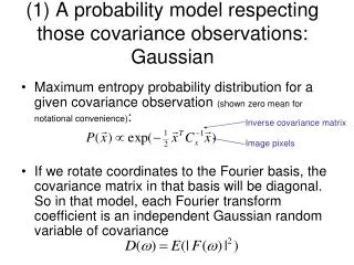
1. (1) A probability model respecting those covariance observations: Gaussian • Maximum entropy probability distribution for a given covariance observation (shown zero mean for notational convenience): • If we rotate coordinates to the Fourier basis, the covariance matrix in that basis will be diagonal. So in that model, each Fourier transform coefficient is an independent Gaussian random variable of covariance Inverse covariance matrix Image pixels

2. Power spectra of typical images Experimentally, the power spectrum as a function of Fourier frequency is observed to follow a power law. http://www.cns.nyu.edu/pub/eero/simoncelli05a-preprint.pdf

3. Random draw from Gaussian spectral model http://www.cns.nyu.edu/pub/eero/simoncelli05a-preprint.pdf

4. Noise removal (in frequency domain), under Gaussian assumption Observed Fourier component Power law prior probability on estimated Fourier component Estimated Fourier component Posterior probability for X Variance of white, Gaussian additive noise Setting to zero the derivative of the the log probability of X gives an analytic form for the optimal estimate of X (or just complete the square):

5. Noise removal, under Gaussian assumption (1) Denoised with Gaussian model, PSNR=27.87 With Gaussian noise of std. dev. 21.4 added, giving PSNR=22.06 original (try to ignore JPEG compression artifacts from the PDF file) http://www.cns.nyu.edu/pub/eero/simoncelli05a-preprint.pdf

6. (2) The wavelet marginal model Histogram of wavelet coefficients, c, for various images. http://www.cns.nyu.edu/pub/eero/simoncelli05a-preprint.pdf Parameter determining peakiness of distribution Parameter determining width of distribution Wavelet coefficient value

7. Random draw from the wavelet marginal model http://www.cns.nyu.edu/pub/eero/simoncelli05a-preprint.pdf

8. And again something that is reminiscent of operations found in V1…

9. An application of image pyramids:noise removal

10. Image statistics (or, mathematically, how can you tell image from noise?) Noisy image

11. Clean image

12. Pixel representation, image histogram

13. Pixel representation, noisy image histogram

14. bandpassed representation image histogram

15. Pixel domain noise image and histogram

16. Bandpass domain noise image and histogram

17. But want the bandpass image histogram to look like this Noise-corrupted full-freq and bandpass images

18. By definition of conditional probability P(x, y) = P(x|y) P(y) The parameters you want to estimate Constant w.r.t. parameters x. Likelihood function Prior probability What you observe Bayes theorem P(x, y) = P(x|y) P(y) so P(x|y) P(y) = P(y|x) P(x) P(x, y) = P(x|y) P(y) so P(x|y) P(y) = P(y|x) P(x) and P(x|y) = P(y|x) P(x) / P(y) Using that twice

19. y P(x) P(y|x) P(y|x) P(x|y) Bayesian MAP estimator for clean bandpass coefficient values Let x = bandpassed image value before adding noise. Let y = noise-corrupted observation. By Bayes theorem y = 25 P(x|y) = k P(y|x) P(x) P(x|y)

20. Bayesian MAP estimator Let x = bandpassed image value before adding noise. Let y = noise-corrupted observation. By Bayes theorem y = 50 P(x|y) = k P(y|x) P(x) y P(y|x) P(x|y)

21. Bayesian MAP estimator Let x = bandpassed image value before adding noise. Let y = noise-corrupted observation. By Bayes theorem y = 115 P(x|y) = k P(y|x) P(x) y P(y|x) P(x|y)

22. P(x|y) P(x) P(y|x) y y = 25 y = 115 y P(y|x) For small y: probably it is due to noise and y should be set to 0 For large y: probably it is due to an image edge and it should be kept untouched P(x|y)

23. MAP estimate, , as function of observed coefficient value, y Simoncelli and Adelson, Noise Removal via Bayesian Wavelet Coring http://www-bcs.mit.edu/people/adelson/pub_pdfs/simoncelli_noise.pdf

24. (1) Denoised with Gaussian model, PSNR=27.87 With Gaussian noise of std. dev. 21.4 added, giving PSNR=22.06 original (2) Denoised with wavelet marginal model, PSNR=29.24 http://www.cns.nyu.edu/pub/eero/simoncelli05a-preprint.pdf

25. M. F. Tappen, B. C. Russell, and W. T. Freeman, Efficient graphical models for processing images IEEE Conf. on Computer Vision and Pattern Recognition (CVPR) Washington, DC, 2004.

26. Motivation for wavelet joint models Note correlations between the amplitudes of each wavelet subband. http://www.cns.nyu.edu/pub/eero/simoncelli05a-preprint.pdf

27. Statistics of pairs of wavelet coefficients Contour plots of the joint histogram of various wavelet coefficient pairs Conditional distributions of the corresponding wavelet pairs http://www.cns.nyu.edu/pub/eero/simoncelli05a-preprint.pdf

28. Gaussian scale mixture model simulation observed (3) Gaussian scale mixtures Wavelet coefficient probability A mixture of Gaussians of scaled covariances z is a spatially varying hidden variable that can be used to (a) Create the non-gaussian histograms from a mixture of Gaussian densities, and (b) model correlations between the neighboring wavelet coefficients.

29. (1) Denoised with Gaussian model, PSNR=27.87 (2) Denoised with wavelet marginal model, PSNR=29.24 With Gaussian noise of std. dev. 21.4 added, giving PSNR=22.06 original (3) Denoised with Gaussian scale mixture model, PSNR=30.86 http://www.cns.nyu.edu/pub/eero/simoncelli05a-preprint.pdf