Abstract

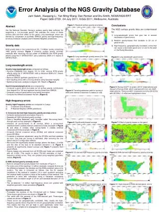
1. Figure 1: Residual surface gravity anomalies • Conclusions • The NGS surface gravity data are contaminated by: • Long-wavelength errors that give rise to several decimeters of geoid errors. • Relative gravity-biases that translate to 20 cm of geoid errors. • High-frequency, geographically-correlated, errors that can cause a decimeter geoid error on and to the west of the Rocky Mountains. Abstract Are the National Geodetic Survey’s surface gravity data sufficient for supporting a 1cm-accurate geoid? We evaluate the errors of these surface data and their effect on the geoid. Long wavelength errors are derived by comparison to synthetic GRACE gravity and high-frequency errors by crossover analysis and K-Nearest-Neighbor predictions. Gravity data NGS gravity data in the conterminous US, 1.4 Million points comprising 1489 gravity surveys. Figure 1 presents surface gravity anomaly residuals after removing the full power of EGM2008 and RTM gravity effects using the 3” SRTM-DTED1 and a reference DEM of 5’ means of SRTM-DTED1. Figure 2: Long wavelength gravity errors (2 to 120) Figure 3: Long wavelength geoid errors • Long wavelength errors • Gravity long wavelength errors computed as follows: • Remove EGM2008 from degree 121 to 2160, remove RTM gravity effects using the 3” SRTM-DTED1 with a reference DEM of 5’’ means of SRTM-DTED1. • Remove GRACE-synthetic gravity from 2-120. • Grid resulting errors with a moving window using Gaussian weights • Spherical harmonic analysis to degree 120. Result in Figure 2. • Geoid long wavelength errors are computed by: • Compute a geoid which truncates out all surface gravity contributions from degree 2 to 120 and replaces them by those from GRACE. • Compute a second geoid without any kernel truncation. • Compute the difference between the two (Figure 3) Error Analysis of the NGS Gravity Database Jarir Saleh, Xiaopeng Li, Yan Ming Wang, Dan Roman and Dru Smith, NOAA/NGS/ERT Paper: G06-2729 , 04 July 2011, IUGG 2011, Melbourne, Australia Figure 5: Survey # 4277 (in green, 22137 observations) and the part of Survey 2094, which overlaps with it (in red, 8425 observations). There are 4601 crossovers but only 230 ECOs with |ECOEs| > 5 mGal are highlighted in blue. Figure 4: Traveling salesman path for survey # 9443 and internal crossovers it creates (in red). • High-frequency errors • Gravity high-Frequency errors are computed in 2 ways: • Crossover (CO) Analysis • K-Nearest-Neighbor (KNN) predictions. • 1) Crossover-derived high-frequency gravity anomaly errors: • Compute residual gravity anomalies (Figure 1). • Separate all 1489 individual gravity surveys. • Pass a “travelling Salesman” path, hereafter called “the survey track”, through each survey (example in Figure 4). • Intersect all survey-tracks of all surveys. When a survey-track intersects itself it creates internal crossovers (ICOs) (example in Figure 4) and when it crosses other survey-tracks it creates external crossovers (ECOs) (example in Figure 5). • Compute internal crossover errors (ICOEs) and external crossover errors (ECOEs). • Compute a crossover adjustment using the ECOEs and their statistics as input. One bias per survey is estimated, after removing the one datum and 217 configuration defects. • We found 244 significantly biased surveys (where the |bias| > 2 mGal and the ratio of the bias to its standard deviation > 2). Figure 6 presents all significantly biased surveys and Figure 7 presents their geoid effects. • Gravity biases are removed from all ECOEs and these are combined with all ICOEs. This results in about 750,000 estimates of high –frequency gravity errors. They are gridded using weighted geometric means (Figure 8). • 2) KNN–derived gravity anomaly errors • Remove all significant gravity biases from residuals of Figure 1. • For every one of the resulting 1.4 million residuals, compute its error as the difference between the residual and the KNN-predicted value at its location. The later is computed as follows. Use the 39 nearest neighbors of the residual in question (10 in each quadrant excluding the residual itself) to predict a value at the location of that residual. The prediction is done with collocation using a Gaussian covariance function with correlation length of 25 km and standard deviation of 1.5 mGal. • The so-obtained 1.4 million high-frequency errors are gridded with weighted geometric mean procedure (Figure 9). • Geoid high-frequency errors: • Propagate the squares of the CO-derived grid in Stokes’ integral. Three-sigma geoid errors are shown in Figure 10. • The same with the squares of the KNN-derived grid. Three-sigma values are shown in Figure 11. • These errors are geographically correlated. Also, clearly the high-frequency gravity errors (Figures 8 & 9) are geographically correlated. This means that they are (at least in part) systematic rather than random. Thus, simple error propagation in Stokes’ may not apply. Figure 6: Significantly biased surveys Figure 7: Effect of gravity biases on the geoid Figure 8: CO-derived high-frequency gravity-anomaly errors Figure 9: KNN-derived high-frequency gravity-anomaly errors Figure 10: High-frequency CO-derived geoid errors Figure 11: High-frequency KNN-derived geoid errors