Requirements to a Line Smoothing Method

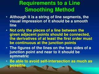
1. Requirements to a Line Smoothing Method • Although it is a string of line segments, the visual impression of it should be a smooth line • Not only the pieces of a line between the given adjacent points should be connected, the derivatives of at least the first order must be continuous at the junction points • The figures of the lines on the two sides of a junction point and near to it should be symmetric • Be able to avoid self-intersection as much as possible

2. Piecewise Line Smoothing Using Third Order Polynomials with Derivatives from Five Points 五点求导分段三次多项式曲线光滑法

3. Third Order Polynomials with Derivatives from Five Points (1) • The basic principle of this method is to set up a third order polynomial equation for a curve between two successive points, and it is demanded that the whole line has the continuous first order derivatives to insure the smoothness of the line. • The first order derivatives on each of the two successive points is determined by this point plus last two points and next two points (5 points altogether).

4. Third Order Polynomials with Derivatives from Five Points (2) • The stipulated geometric condition for the tangential line passing through the middle point: P1 P5 P2 P4 P3 C A D B

5. Third Order Polynomials with Derivatives from Five Points (3) • Through mathematical derivation, the derivative t3 on the point P3 can be expressed as:

6. Third Order Polynomials with Derivatives from Five Points (4) (a02+b02)1/2 In order to be convenient, we use cosθ3and sinθ3 for t3(i.e., tgθ3), and the numerator and the denominator of the expression for t3 are seen as the two edges of a right triangle: b0 θ a0 When w2=w3=0, cos θ3and sin θ3 are uncertain, let w2=w3=1

7. Third Order Polynomials with Derivatives from Five Points (5) Let the third order polynomial equations between the two successive points Pi and Pi+1 be: x=p0+p1z+p2z2+p3z3 y=q0+q1z+q2z2+q3z3 In these equations, pi, qi (i=0,1,2,3) are constants, z is the parameter, when the curve is being generated from Pi (xi, yi) to Pi+1 (xi+1, yi+1), z is changing from 0 to 1.

8. Third Order Polynomials with Derivatives from Five Points (6) These equations should satisfy the following conditions: When z=0, x=xi, y=yi, dx/dz=rcosθi, dy/dz=rsinθi, When z=1, x=xi+1, y=yi+1, dx/dz=rcosθi+1, dy/dz=rsinθi+1. Where r=[(xi+1-xi)2+(yi+1-yi)2]1/2 Pi+1 θi Pi θi+1

9. Third Order Polynomials with Derivatives from Five Points (7) From these conditions, pi and qi (i=0,1,2,3) can be uniquely defined: p0=xi p1=rcosθi p2=3(xi+1-xi)-r(cosθi+1+2cosθi) p3=-2(xi+1-xi)+r(cosθi+1+cosθi) q0=yi q1=rsinθi q2=3(yi+1-yi)-r(sinθi+1+2sinθi) q3=-2(yi+1-yi)+r(sinθi+1+sinθi)

10. Third Order Polynomials with Derivatives from Five Points (8) • Supplement of two points on each end for an open line – Suppose that the first three given points (x3,y3), (x4, y4), (x5, y5), and the two points to be supplied (x2,y2) and (x1,y1) are all on the following line: x=g0+g1z+g2z2 y=h0+h1z+h2z2

11. Third Order Polynomials with Derivatives from Five Points (9) where gk, hk (k=0,1,2) are constants, z is the parameter, and suppose that when z=j, x=xj, y=yj (j=1,2,3,4,5), then: x2=3x3-3x4+x5 x1=3x2-3x3+x4 y2=3y3-3y4+y5 y1=3y2-3y3+y4 The supplement of the points after the last given point is similar to this.

12. Third Order Polynomials with Derivatives from Five Points (10) • Advantages: • To be strict mathematically • Relatively simple in calculation • The resulted curve can pass through every given point exactly while has the continuous first order derivatives everywhere on the line • When given points are relatively dense, the resulted curve will be satifactory

13. Third Order Polynomials with Derivatives from Five Points (11) • Disadvantages: • The graphic representation would not be ideal at the place of the sudden turning of the curve • For the successive zigzag meanders, the curve sometimes intersects with itself

14. Piecewise Line Smoothing Using Third Order Polynomials with Derivatives from Three Points 三点求导分段三次多项式曲线光滑法

15. Third Order Polynomials with Derivatives from Three Points (1) The basic principle of this method is similar with the method used in the piecewise line interpolation using the three order polynomial with derivatives from five points. The main difference lies in the method of determination for the derivatives.

16. Third Order Polynomials with Derivatives from Three Points (2) • The derivative on every given point is determined by the relative positions of the last and next points to this point. Therefore, three successive points are used to calculate the derivative of the curve on the middle point • Let the three points be Pi-1, Pi, Pi+1, their coordinates are (xi-1, yi-1), (xi, yi), (xi+1, yi+1) respectively

17. Third Order Polynomials with Derivatives from Three Points (3) Suppose that there is a point M (xm, ym) on the

18. Third Order Polynomials with Derivatives from Three Points (4) Y Pi E Ti F αi Pi+2 Pi-1 M αi+1 Pi+1 Ti+1 O X

19. Third Order Polynomials with Derivatives from Three Points (5) The slope of the line segment PiM is: KPiM = (ym-yi) / (xm-xi) therefore, the slope of the tangential line on point Pi is: KEF = -1 / KPiM Let thedirection of EF be identical with the moving direction of the curve.

20. Third Order Polynomials with Derivatives from Three Points (6) After the quadrant judgement, the angle αbetween the directed line EF and the X-axis can be uniquely determined within the range of 0 - 2π. tgαis the first order derivative at the point Pi on the curve. All the derivatives tgαi (i=2,3,...,N-1) can be calculated in this way.

21. Third Order Polynomials with Derivatives from Three Points (7) The establishment of the parametric equations of the third order polynomials is just like the way for setting up the equations for the third order polynomials with derivatives from five points.

22. Third Order Polynomials with Derivatives from Three Points (8) Attention must be paid to: • For an open line, the derivative of the first or last point can be seen as the slope of the tangential line on the first or last point of a circle or a parabolic line which passes through the first three points or the last three points • For special cases such as three successive points locate on a same straight line, or the slope of the line segment KPiM is nearly infinitive, judgement and assignment must be made in advance

23. Third Order Polynomials with Derivatives from Three Points (9) r can be changed in order to change the tightness of the curve. Therefore, in order to regulate the tightness of the curve in time, the two angles which are formed by the string Pi-1PiPi+1Pi+2 are used as the components of the weight function to regulate the value of r, called r’: r’ = r · |(1-z)sinβi+zsinβi+1|

24. Third Order Polynomials with Derivatives from Three Points (10) βi βi+1 r’ = r · |(1-z)sinβi+zsinβi+1|

25. Third Order Polynomials with Derivatives from Three Points (11) • Advantages: • This method can give satisfactory result even if the given points are distributed relatively sparse • The curve passes through all the given points • The first order derivatives are continuous at everywhere on the curve • Graphical symmetry near every point • The ability to avoid self intersection • To be simple in mathematic principle and easy to write the program

26. Third Order Polynomials with Derivatives from Three Points (12)

27. Questions for Review (1) • What are the general requirements for line smoothing? • What are the advantages and disadvantages of weighted average of normal axis parabolic lines? • What are the differences between the methods of piecewise line smoothing using third order polynomials with derivatives from five and from three points?

28. Questions for Review (2) • Please describe the concrete steps of line smoothing using third order polynomials with derivatives from three points. • How are the derivatives calculated using the “five point method“? • How are the derivatives calculated using the “three point method“? • What are the frame conditions with respect to the change of parameter z in the third order polynomial line smoothing?